Estimating the Entrance Length of Channel Flow#
Prepared by: Stephen Cini (scini@nd.edu) and David Gazzo (dgazzo@nd.edu)
Reference: Problem 4.5, pg. 210, Transport Phenomena in Biological Systems by Truskey et al. (ISBN 978-0-13-156988-1)
Intended Audience: This problem is intended for Chemical and Biomolecular Engineering juniors and seniors from the University of Notre Dame who are either enrolled in or have taken Transport.
Learning Objectives#
After studying this notebook, completing the activities, and asking questions in class, you should be able to:
Apply integration techniques to ordinary differential equations using Python.
Properly graph and visualize data using
matplotlib.Apply integration techniques to realistic scenarios using Python tools such as
scipy.integrate.
Coding Resources#
Relevant Modules in Class Website:
# load libraries
import numpy as np
import matplotlib.pyplot as plt
from scipy import integrate
Problem Statement:#
Homework Problem
Complete the following problem outside of class to practice the concepts discussed.
Developing flow within a channel can be examined with boundary layer theory. Consider a rectangular channel of height \(H\) and width \(w\) such that \(w >> H\).
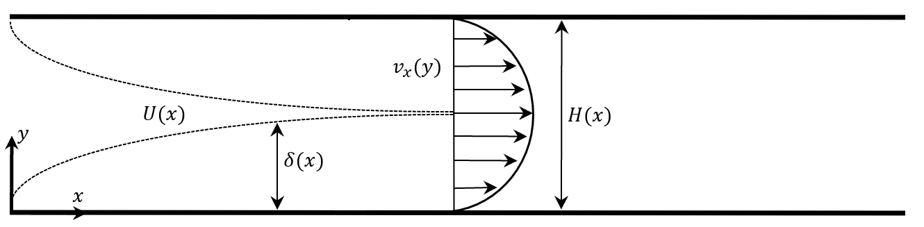
The velocity field in the entrance depends upon the x and y directions. As shown in the figure below, a boundary layer develops as flow enters the channel: Once the boundary layer has grown to equal H/2, the flow is fully developed.
1. Estimating Entrance Length#
As a first approximation, assume that the boundary layer is described by the results for flow over a flat plate. That is, the development of the boundary layer \(δ\) is given by
where,
Develop an expression for the entrance length in terms of the channels Reynolds number, \(Re_x=2ρUH/μ = 2ρQ/wμ\), where \(〈v〉\) is the average velocity in the channel.
Show that the entrance length \(Le\) is equal to \(0.005ReH\).
Submit your answer and written work via Gradescope.
2. More Accurate/Rigorous Method#
2a. Normalize the expression on paper#
The analysis in Question 1 assumes that \(U(x) = U_o = 〈v〉\). But in fact, the free-stream velocity changes as the boundary layer grows in the channel. Therefore, assuming a linear velocity profile, \(v_x=\frac{U_xy}{δ}\), in the boundary layer, and utilizing the von Karman momentum integral equation,
and the fact that the flow rate \(Q\) is constant, the following expression for the growth of the boundary layer can be derived:
Manipulate this expression so that it can be integrated numerically. Hint: normalize it and keep symmetry in mind.
Submit your answer and written work via Gradescope.
2b. Numerically integrate the normalized expression#
Using the normalized form of the differential equation, use scipy.integrate.solve_ivp to numerically integrate the expression and find the value of x where \(δ\) is fully developed.
For more information on how to use scipy.integrate, click here to go to the relevant section of the class website.
def entrance(d, x, Re=1):
    """Solving for the entrance length of the tube with non constant velocity
    Args:
        d: δ_star; Normalized δ; partial derivative wrt x or y (numpy array)
        x: x_star; Normalized x; position along channel (numpy array)
        Re: Reynolds number, constant dimensionless quantity used to show
        turbulence or roughness of flow. Set to unity as default value (float)
    Returns:
        dxdy: Normalized expression for the entrance length
    """

    # assume Re is at unity for the example

    # Add your solution here

    return dxdy
# Integrate the solution in scipy using defined function

# Add your solution here
2c. Plot the results#
Plot the resulting data to show the behavior of the integrated expression.
For more information on how to use matplotlib to make publication quality plots, click here to go to the relevant section of the class website.
# Plot the integrated expression

fig = plt.figure(figsize=(5, 3), dpi=200)  # formats the plotted figure

# Add your solution here

# Format for publication quality
plt.xlabel("x*/Re [dimensionless]", fontsize=16, fontweight="bold")
plt.ylabel("\u03B4* [dimensionless]", fontsize=16, fontweight="bold")
plt.xticks(fontsize=15)
plt.yticks(fontsize=15)
plt.grid()
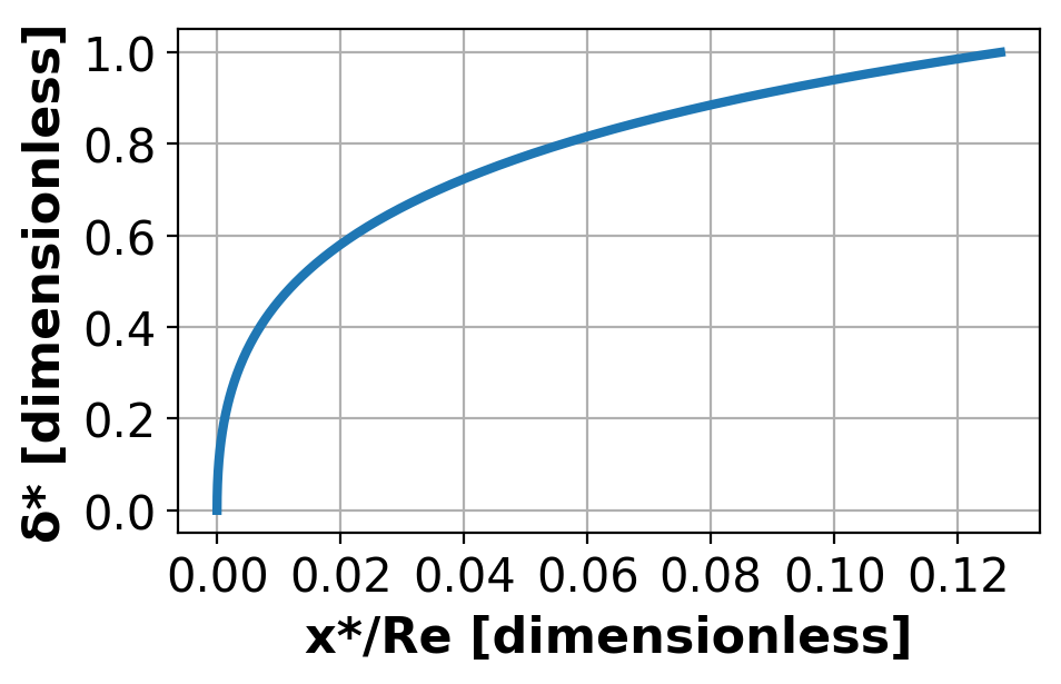
2d. Define the entrance length#
At what value of x does the boundary layer become fully developed?
Hint: What is the coordinate where \(δ\) = 1?
Store your solution as a numpy array labelled Le.
# Add your solution here

# Print Value
print("Le (x @ δ*=1) =", Le)  # we want to know the dimensionless
# length at which del is 1 since this will give us our entrance length where
# flow is stil developing
Le (x @ δ*=1) = 0.12694690354738747
2e. Define an equation for Le using new value#
Using the obtained value of Le, make a general expression for the entrance length similar to the expression derived in part 1.
Hint: The value obtained for Le is dimensionless.
Submit your answer and written work via Gradescope.
2f. Comparing integration methods#
Compare your previous results using the RK45 integration method with alternative methods.
Define your equation as methods.
For more information on other integration methods for scipy.integrate, click here to go to the relevant section of the class website. Further detail into integration methods for scipy.integrate, is also provided in the documentation here.
# make a list of methods
methods = ["RK23", "RK45", "DOP853"]

# loop through methods for best
for i in methods:
    print("Using method", i)

    # Add your solution here

    # print values for each method within loop
    # some solver statistics
    print("Number of RHS function evaluations:", other_methods.nfev)
    # calculated length from each method
    print("Le (x @ δ*=1) =", Le)  # dimensionless
    print("\n")
Using method RK23
Number of RHS function evaluations: 53
Le (x @ δ*=1) = 0.12693195882302588


Using method RK45
Number of RHS function evaluations: 38
Le (x @ δ*=1) = 0.12694690354738747


Using method DOP853
Number of RHS function evaluations: 89
Le (x @ δ*=1) = 0.12694710642481696
3. Discussion and Analysis#
3a. Explain why the equation derived in Question 2e differs from the one obtained in Question 1.#
Discuss in 1-3 sentences.
Answer:
3b. Describe the integration methods used in 2f and how they differ in performance. Was the best method used originally in 2b? Why or why not?#
Discuss in 3-5 sentences.
Answer:
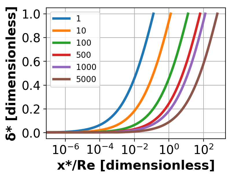
3c. A Reynolds number of 1 was used as a starting point to simulate laminar flow. If the Reynolds number were increased, what would happen to the entrance length? Does it get larger or smaller? Why does this occur?#
Explain your reasoning using the derived equations for Le and the nature of turbulence.
Discuss in 3-5 sentences.
Answer:
To visualize, plot the curve above with the following values of Re:
1, 10, 100, 500, 1000, 5000.
Hints:
Use a lambda function to allow redefinition of Re.
Make a semi-log plot for easier viewing of trend in results.
# Redefine Re in same function from before within a for loop.

# Add your solution here

fig = plt.figure(
    figsize=(4, 3), dpi=200
)  # formats the plotted figure to be larger and clearer

# loop the integration for different values of Re
# plot each iteration inside loop

for i in range(len(Mult_Re)):
    # Add your solution here

    # print values for Le
    print("Le (x @ δ*=1) for Re =", Mult_Re[i], "=", Le)
print("\n")

# labels and publication quality details
plt.xlabel("x*/Re [dimensionless]", fontsize=16, fontweight="bold")
plt.ylabel("\u03B4* [dimensionless]", fontsize=16, fontweight="bold")
plt.xticks(fontsize=15)
plt.yticks(fontsize=15)
plt.grid()
plt.legend()
Le (x @ δ*=1) for Re = 1 = 0.12694690354738747
Le (x @ δ*=1) for Re = 10 = 1.2695003130784555
Le (x @ δ*=1) for Re = 100 = 12.695115409153276
Le (x @ δ*=1) for Re = 500 = 63.47563865495485
Le (x @ δ*=1) for Re = 1000 = 126.95129304465897
Le (x @ δ*=1) for Re = 5000 = 634.7565284345559