10.1. Basic Ideas of Probability#
10.1.1. Learning Objectives#
After attending class, completing these activities, asking questions, and studying notes, you should be able to:
Understand basic probability vocabulary.
Be able to calculate the probabilities of various conditional/unconditional events.
Be familiar with the axioms of probability.
Know when and how to use permutation versus combination calculations.
Be able to evaluate calculations using the multiplication rule, Bayes’ rule, and the Law of Total Probability.
10.1.2. Definitions#
Sample Space: all possible outcomes of an experiment
Subset: a set each of whose elements is an element of an inclusive set
Event: a subset of the seample space
Example: flipping two coins
Sample space:
H, H
H, T
T, H
T, T
Example event: H, T
10.1.3. Combining Events#
Consider two events: \(A\) and \(B\)
Union: “\(A\) or \(B\) “ ; \(A \cup B\)
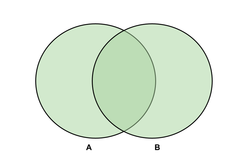
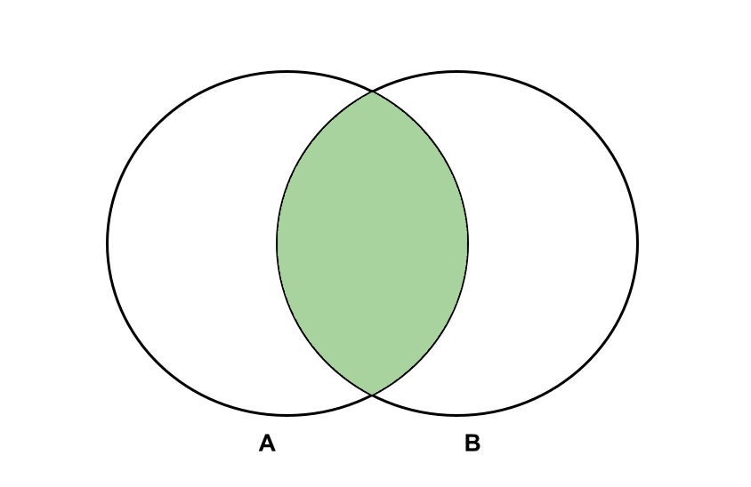
Intersection: “\(A\) and \(B\) “ ; \(A \cap B\)
Complement: “not \(A\) “ ; \(A^c\) or \(\rightharpoondown A\)
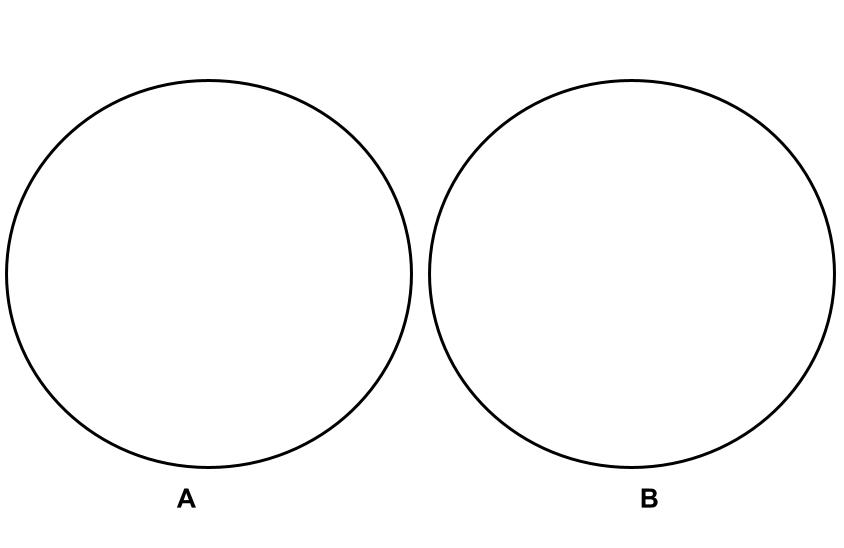
Mutually Exclusive Events: no outcomes in common
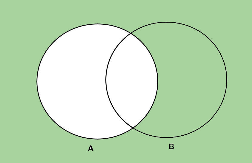
Home Activity
What is shown in the venn diagram below?
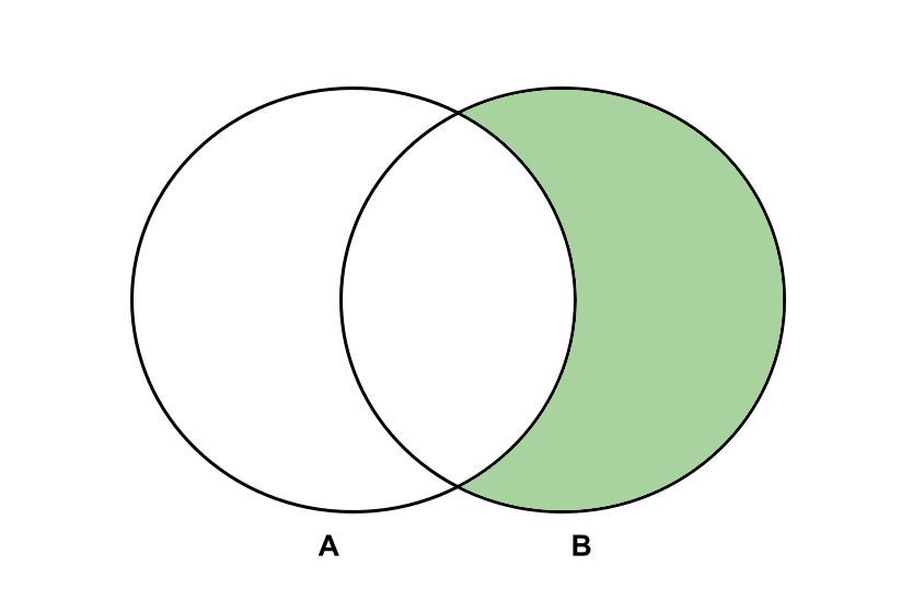
Record your answer as a letter string assigned to ans1 in the cell below:
a. \(A^c \cap B\)
b. \(A \cap B^c\)
c. \(A^c \cup B\)
d. \(A \cup B^c\)
# Add your solution here
10.1.4. Probabilities#
Given an experiment (random process) and any event…
\(P(A)\) - probability an event occurs
\(P(A)\) is proportional to the number of times \(A\) would occur if the experiment was repeated many times.
Example: flipping two fair coins (all events equally likely)
I could define the experiment differently, and instead just count the number of heads:
Sample space: 0, 1, 2
10.1.5. Axioms of Probability#
Let \(S\) be a sample space. \(P(S) = 1\)
For any event \(A\), \(0 = P(A) \leq 1\)
If \(A\) and \(B\) are mutually exclusive (no intersection in Venn diagram)…
In general,
For any event A,
10.1.6. Permutations#
With permutations, order matters!
Example: How many ways to schedule 4 in-class group presentations? The teams are A, B, C, D.
4 x 3 x 2 x 1 = 4! = 24
More General Case: How many ways to schedule 2 teams from 5 are possible? (As in AB, BA, AC, CA…)
An easy way to remember the order of subscripts for permutations is “n choose k”.
10.1.7. Combinations#
With combinations, order does not matter!
Example: Given a list of 5 burger toppings (A, B, C, D, E), how many ways to choose 2?
AB, AC, AD, AE, BC, BD, BE, CD, CE, DE = 10
More General Case:
So for the above example…
We will use permutations and combinations to estimate probabilities of events such as…
winning the lottery
observing a molecular system in a specific state
10.1.8. Conditional Probability#
Conditional Probability: based on only a part (subset) of the sample space, the probability of one event occurring in the presence of a second event
Example: You look out the window and notice it looks cloudy. You’re wondering if it’s going to rain and get the grass wet. The following table gives the distribution of outcomes for the last 100 days so that you can make an informed guess about today’s weather.
|
Rain-sky (R) |
Clear-sky (C) |
total |
|---|---|---|---|
Wet-grass (W) |
20 |
10 |
30 |
Dry-grass (D) |
5 |
65 |
70 |
total |
25 |
75 |
100 |
What is the probability it’s raining given the grass is dry?
\(P\)(raining | dry grass) = \(\frac{5}{70}\)
More General Case:
Let \(A\) and \(B\) be events with \(P(B) \neq 0\).
So for the above example…
General Formulas:
Conditional Probability:
Conditional Probability Mass Function:
Conditional Probability Density Funtion:
Conditional Expectation:
Example: CD Cover Below are data of the length and width of CD covers:
length (x) |
width (y) |
\(\rho\)(X=x and Y=y) |
|---|---|---|
129 |
15 |
0.12 |
129 |
16 |
0.08 |
130 |
15 |
0.42 |
130 |
16 |
0.28 |
131 |
15 |
0.06 |
131 |
16 |
0.04 |
Compute \(P_{Y | X}(y | 130)\).
Possibility 1: y=15 (given x=130)
Possiblity 2: y=16 (given x=130)
Compute \(E[Y | X=130]\).
Unconditional probability:
This is the probability of it raining without any other subsets to consider, just out of the total sample space.
10.1.9. Independence#
Two events \(A\) and \(B\) are independent if…
1. \(P(B | A) = P(B)\) & \(P(A | B) = P(A)\) (equivalent statements)
given
\(P(A) \neq 0\) & \(P(B) \neq 0\)
2. \(P(A) = 0\) & \(P(B) = 0\)
Independence means knowing \(A\) does not tell you anything about \(B\) and vice versa.
Question: Are “raining” and “grass wet/dry” indepndent?
10.1.10. Multiplication Rule#
If \(P(B) \neq 0\), then \(P(A \cap B) = P(B)P(A | B)\)
If \(P(A) \neq 0\), then \(P(A \cap B) = P(A)P(B | A)\)
10.1.11. Law of total probability#
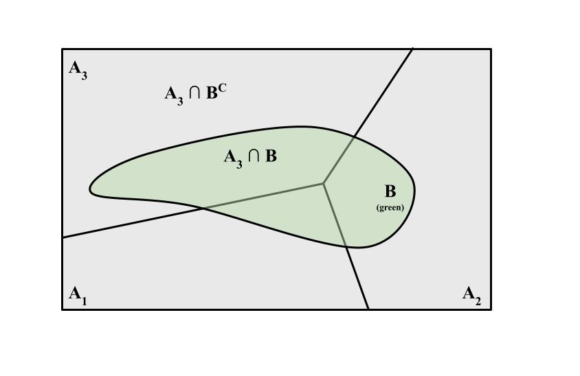
If \(A_1...A_n\) are mutually exclusive (no overlap) and exhaustive, i.e.
and \(B\) is any event, then
10.1.12. Bayes’ Rule#
In general,
So how do we convert between conditional probabilities? We use Bayes’ rule…
Let’s return to the rain and grass example.
Now let’s verify that Bayes’ rule works for the rain and grass example…
As expected, it works!
Example: 0.5% of people in a community have a disease.
If a person has a disease there is a 99.9% probability they will test positive.
If a person does not have a disease, there is a 1% probability they will test positive.
Calculate the probability that if someone tests positive, they are actually sick.
Bayes’ rule:
10.1.13. Expected Value/Mean of Functions#
We will use the following formulas to compute the average ofo a function \(h(x)\):
Discrete:
What is \(\mu_{h(x)}\) when \(h(x) = (x-\mu_x)^2\)?
Answer: variance