13.5. Hypothesis Testing Basics#
Further Reading: §6.1, §6.2, and §6.4 in Navidi (2015)
13.5.1. Learning Objectives#
After studying this notebook, attending class, completing the home activities, and asking questions, you should be able to:
Use a confidence interval to perform hypothesis testing
Apply the 5-step hypothesis testing procedure
Identify null and alternative hypotheses from a problem description
Calculate test statistic
Draw “area under curve” that corresponds to P-value for a given set of hypotheses
# load libraries
import scipy.stats as stats
import numpy as np
import math
import matplotlib.pyplot as plt
13.5.2. Main Idea#
Using a sample, draw inference about a scientific hypothesis involving the population mean. (Engineers are sometimes interested in inference about the population variance too. We will learn about these flavors of hypothesis testing in the Flavors of Hypothesis Testing notebook. Please note that hypothesis testing is not limited to the population mean.)
13.5.3. Motivating Example: Catalyst Lifetime#
Story
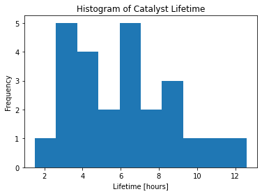
As a process engineer, you would like to infer if a new catalyst (data shown below/also in last notebook) has a longer life than current catalyst (5.7 hours) used in our company’s process.
# Catalyst example data
lifetime = [3.2, 6.8, 4.2, 9.2, 11.2, 3.7, 2.9, 12.6, 6.4, 7.5, 8.6,
            4.5, 3.0, 9.6, 1.5, 4.5, 6.3, 7.2, 8.5, 4.2, 6.3, 3.2, 5.0, 4.9, 6.6]

# Compute the mean and standard deviation
xbar = np.mean(lifetime)
s = np.std(lifetime)

# Plot lifetime data
plt.hist(lifetime)
plt.title("Histogram of Catalyst Lifetime")
plt.xlabel("Lifetime [hours]")
plt.ylabel("Frequency")
plt.show()

Sample Statistics
print("Lifetime Average:",round(xbar,2),"hours")
print("Lifetime Standard Deviation: {:.2f} hours".format(s))
Lifetime Average: 6.06 hours
Lifetime Standard Deviation: 2.72 hours
Key Question
The mean sample lifetime is 6.06 hours, which is much better than the 5 hour goal. Here are two possible interpretations of the data:
The population mean (new catalyst lifetime) is actually 5.7 hours or less. The sample mean is higher because of random variations in the experiment (sampling from the population).
The population mean is actually 5.7 hours or greater, and the sample reflects this fact.
We will use hypothesis testing to discern between these two possible explanations.
Mathematically, we want to draw a conclusion about the mean catalyst lifetime, i.e., the expected value of the population distribution.
13.5.4. Null and Alternative Hypotheses#
Null Hypothesis (option 1 above, denoted \(H_0\)): Effect indicated by the sample is due to random variations.
Alternative Hypothesis (option 2 above, denoted \(H_1\) or \(H_a\)): Effect indicated by the sample is real.
13.5.5. Hypothesis Testing Procedure#
Define \(H_0\) and \(H_1\).
Assume \(H_0\) to be true.
Compute the test statistic.
Compute the P-value.
State conclusions.
We will follow these steps whenever doing hypothesis testing in this class. We will now walk through the catalyst lifetime example.
13.5.5.1. Step 1. Define Hypotheses.#
13.5.5.2. Step 2. Assume \(H_0\) is True.#
We do not need to write anything for this step. But it is important to remember this assumption for the remaining calculations.
13.5.5.3. Step 3. Compute the Test Statistic.#
We do not know the population standard deviation, so we will use a t-statistic.
tscore = (xbar - 5.7)/(s / math.sqrt(len(lifetime)))
print("t = ",tscore)
t = 0.6694840523966666
13.5.5.4. Step 4. Calculate P-Value.#
The P-value tells us the probability of observing a sample as or more extreme than the current one if the null hypothesis is true. (Remember Step 2.)
We can calculate the P-Value by integrating the area under the t-distribution (or normal distribution). I strongly recommend drawing a picture of a z-/t-distribution and shading the area under the curve that corresponds with the P-value. This is essential to not make a sign mistake when using cdf(). The integral is intractable, so we will use Python or a look-up table.
# You'll want to draw a picture whenever connecting a P-value to the cdf() function in Python
pval = 1 - stats.t.cdf(tscore, len(lifetime)-1)
print("P-value:",pval)
P-value: 0.2547883922583275
13.5.5.5. Step 5. State Conclusions#
The P-value is 0.25, which is greater than 0.05, so we fail to reject the null hypothesis. We cannot conclude the new catalyst has a mean lifetime greater than 5.7 hours.
Important Ideas:
The smaller the P-value, the more certain we are that \(H_0\) is false.
The larger the P-value, the more plausible \(H_0\).
We can never be certain the \(H_0\) is true. Thus we never conclude “accept the null hypothesis”.
We can only conclude to reject the null hypothesis or fail to reject the null hypothesis. We can never be certain the \(H_0\) is true, and thus never say “accept the null hypothesis”.
Rule of thumb is to reject \(H_0\) whenever \(P \leq 0.05\), but this has no scientific basis.
The P-value is NOT the probability \(H_0\) is true. (To make this statement, we would need Bayesian statistics.)
Statistical Significance. For \(P \leq \alpha\) and \(0 < \alpha < 1\), people often say:
The results of the test are statistically significant at the 100\(\alpha\)% level.
The null hypothesis is rejected at 100\(\alpha\)% level.
13.5.6. Summary of Hypotheses and P-Values#
Null Hypothesis |
Alternate Hypothesis |
P-Value |
|---|---|---|
\(H_0: \mu \leq \mu_0\) |
\(H_a: \mu > \mu_0\) |
Area to the right of \(z\) (or \(t\)) |
\(H_0: \mu \geq \mu_0\) |
\(H_a: \mu < \mu_0\) |
Area to the left of \(z\) (or \(t\)) |
\(H_0: \mu = \mu_0\) |
\(H_a: \mu \neq \mu_0\) |
Sum of the areas in the tails cut off by \(z\) and \(-z\) (or \(t\) and \(-t\)) |
Coda: Confidence Intervals and Hypothesis Testing are Closely Related
13.5.7. Review Hypothesis Testing Conclusions#
Home Activity
At a minimum, skim §6.2 (pg. 409 - 414) in Navidi (2015).
13.5.7.1. Test your Understading#
We want to check the calibration of a scale by weighing a standard 10g weight 100 times. Let \(\mu\) be the population mean reading on the scale, so that the scale is in calibration if \(\mu = 10\). A test is made of the hypotheses \(H_0: \mu = 10\) versus \(H_a: \mu \neq 10\).
Home Activity
Answer the following multiple choice questions.
Which of the following is the best interpretation of the conclusion “H\(_0\) is rejected”?
The scale is in calibration.
The scale is not in calibration.
The scale might be in calibration.
Store your answer in the Python integer ans_18a_i.
# Add your solution here
# Removed autograder test. You may delete this cell.
Which of the following is the best interpretation of the conclusion “Failed to reject H\(_0\)”?
The scale is in calibration.
The scale is not in calibration.
The scale might be in calibration.
Store your answer in the Python integer ans_18a_ii.
# Add your solution here
# Removed autograder test. You may delete this cell.
Is it possible to perform a hypothesis test in a way to demonstrate conclusively the scale is in calibration?
Yes
No
Sometimes yes, sometimes no
Store your answer in the Python integer ans_18a_iii.
# Add your solution here
# Removed autograder test. You may delete this cell.
Write a sentence to explain your answer to the last question.
Home Activity Answer:

