11.1. Bernoulli Probability Distribution

Further Reading: §4.1 in Navidi (2015)

11.1.1. Learning Objectives

After studying this notebook, completing the activities, engaging in class, and reading the book, you should be able to:

• Model scientific and engineering problems using the Bernoulli distrubtion.

import numpy as np
from scipy.stats import bernoulli
import matplotlib.pyplot as plt

11.1.2. Definition

The Bernoulli distribution considers a single experiment with two outcomes: “success” or “failure”. The parameter \(p\) encoded the probability of success. This is the simplest discrete distribution and is the building block for many others.

We often write \(X \sim\) Bernoulli(\(p\)), which means random variable \(X\) follows the Bernoulli distribution with parameter \(p\).

Thus the probability mass function is:

Failure: \(p(0) = P(X = 0) = 1 - p\)

Success: \(p(1) = P(X = 1) = p\)

Using the definitions for mean and variance:

\[\mu_X = \sum_x x p(x)\]

\[\sigma_X^2 = \sum_x (x - \mu)^2 p(x)\]

it is easy to show \(\mu_X = p\) and \(\sigma_X^2 = p(1-p)\) for the Bernoulli distribution.

Note

Study Activity: Derive the mean and variance for the Bernoulli distribution.

Home Activity

Read through the python implementation below and note any questions you have.

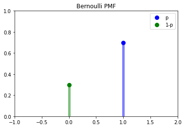
# display the probability mass function
fig, ax = plt.subplots(1, 1)
p = 0.3
x = np.arange(bernoulli.ppf(0.01, p), bernoulli.ppf(0.99, p))
ax.plot(1, bernoulli.pmf(x, p), 'bo', ms=8, label='p')
ax.plot(0,bernoulli.pmf(x,1-p),'go', ms=8, label='1-p')
ax.vlines(1, 0, bernoulli.pmf(x, p), colors='b', lw=5, alpha=0.5)
ax.vlines(0, 0, bernoulli.pmf(x, 1-p), colors='g', lw=5, alpha=0.5)
plt.xlim([-1,2])
plt.ylim([0,1])
plt.legend()
plt.title('Bernoulli PMF')
plt.show()