14.4. Residual Analysis

Further Reading: §7.4 in Navidi (2015), Checking Assumptions and Transforming Data

14.4.1. Learning Objectives

After studying this notebook and your lecture notes, you should be able to:

• Check linear regression error assumptions using residual analysis (plots)

• Compute residual standard error and covariance matrix for fitted parameters

# load libraries
import scipy.stats as stats
import numpy as np
import math
import matplotlib.pyplot as plt

14.4.2. Residual Analysis

Recall the simple linear model:

\[y_i = \beta_0 + \beta_1 x_i + \epsilon_i\]

We are now going to focus on the random observation error \(\epsilon\). In order to perform uncertainty analysis and statistical inference (next notebook), we need to check the following assumptions about the error:

1. The errors \(\epsilon_1\), …, \(\epsilon_n\) are random and independent. Thus the magnitude of any error \(\epsilon_i\) does not impact the magnitude of error \(\epsilon_{i+1}\).

2. The errors \(\epsilon_1\), …, \(\epsilon_n\) all have mean zero.

3. The errors \(\epsilon_1\), …, \(\epsilon_n\) all have the same variance, denoted \(\sigma^2\).

4. The errors \(\epsilon_1\), …, \(\epsilon_n\) are normally distributed.

We will now discuss several strategies to check these assumptions.

14.4.3. Calculate Residuals

We cannot measure \(\epsilon_i\) directly. Instead, we will estimate it using the residual:

\[ \underbrace{e_i}_{\mathrm{residual}} = \underbrace{y_i}_\mathrm{observation} - \underbrace{\hat{y}_i}_{\mathrm{prediction}} \]

We might write \(r_i\) instead of \(e_i\) for residual. Old habit.

# necessary data from previous notebook to calculate residuals
pH = np.array([4.6, 4.8, 5.2, 5.4, 5.6, 5.8, 6.0])
yld = np.array([1056, 1833, 1629, 1852, 1783, 2647, 2131])
b1_ = 737.1014492753624
b0_ = -2090.942028985508

yld_hat = b0_ + b1_ * pH
e_farm = yld - yld_hat
print("Residuals (pounds / acre):")
print(e_farm)

Residuals (pounds / acre):
[-243.72463768  385.85507246 -112.98550725  -37.4057971  -253.82608696
  462.75362319 -200.66666667]

14.4.4. Histogram of Residuals

Assumption 4: Are the residuals normally distributed?

plt.hist(e_farm)
plt.xlabel("Residual (pounds / acre)")
plt.ylabel("Frequency (count)")
plt.show()

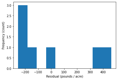
Interpretation Questions:

1. Are there any extreme outliers?

2. (large data sets) Does the histogram look approximately normal?

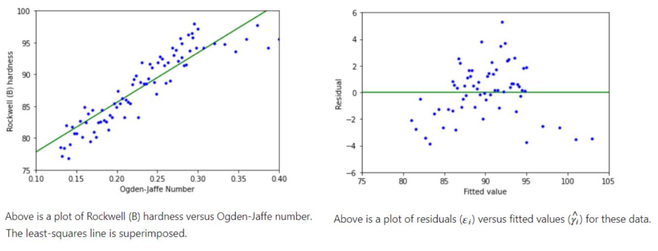
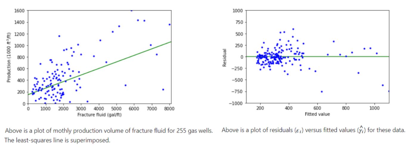
14.4.5. Scatter Plot of Residuals versus Predicted Values

Assumption 1: Are the residuals random and independent?

plt.plot(yld_hat,e_farm,"b.", markersize=20)
plt.xlabel("Predicted Yield (pounds / acre)")
plt.ylabel("Residual (pounds / acre)")
plt.grid(True)
plt.show()

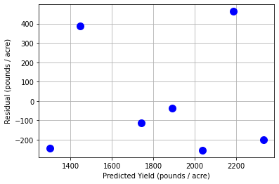
Interpretation Questions:

1. Are there any clear patterns in the residuals?

2. Are there any extreme outliers?

Additional Example

x = np.random.normal(0,20,200)
y = np.random.normal(-4,4,200)
plt.scatter(x,y)
plt.xlabel('Fitted values')
plt.ylabel('Residuals')
plt.show()

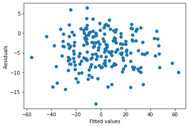
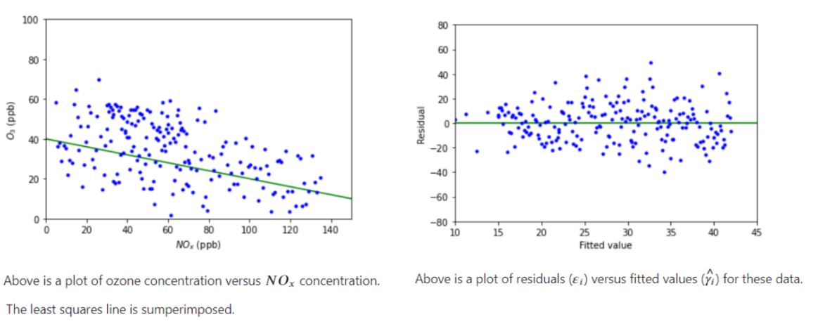
As you can see, there is no significant pattern to this plot and the vertical spread doesn’t vary too much. This is consistent with the linear model assumptions.

14.4.6. Scatter Plot of Residuals versus Independent Variable

Assumption 1: Are the residuals random and independent?

plt.plot(pH,e_farm,"b.",markersize=20)
plt.xlabel("Soil pH")
plt.ylabel("Residual (pounds / acre)")
plt.grid(True)
plt.show()

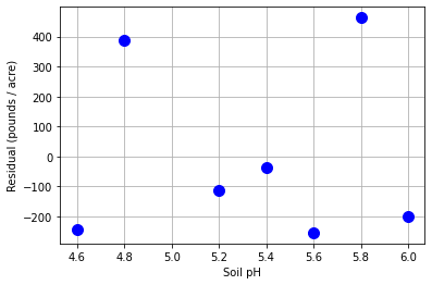
Interpretation Questions:

1. Are there any clear patterns in the residuals?

2. Are there any extreme outliers?

Additional Examples

14.4.7. Scatter Plot of Residuals versus Data Collection Order

If you know the order data were collected, it is critical to create another scatter plot. You need to ensure there are no patterns (correlations) in time.

14.4.8. Scatter Plot of Residuals Squared versus Independent Variable (and Collection Order)

Assumption 3: Do the residuals have the same variance?

plt.plot(pH,e_farm**2,"b.",markersize=20)
plt.xlabel("Soil pH")
plt.ylabel("Residual Squared (pounds / acre)$^2$")
plt.grid(True)
plt.show()

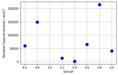
Interpretation Questions:

1. Do the residuals squared grow or shrink as the independent variable increases?

2. Do the residuals squared grow or shrink with collection order?

Additional Examples:

These examples are further explored in the assumption violation notebook.

Example 1:

---

Example 2:

---

Example 3:

14.4.9. What if an assumption is violated?

There are several strategies to try:

1. Try a different model (tranform variables, nonlinear regression)

2. Weighted regression

3. Robust regression

We will discuss 1 and 2 during the next few lectures.

In this notebook we discuss assumption violations in more detail with a few examples.

Class Activity

As an intern, you help run a chemical process 24 times to determine the effect of temperature on yield. The data below are presented in the order of the runs. With a partner, complete the following analysis steps.

temp = np.array([30, 32, 35, 39, 31, 27, 33, 34, 25, 38, 39, 30, 30, 39, 40, 44, 34, 43, 34, 41, 36, 37, 42, 28])
proc_yld = np.array([49.2, 55.3, 53.4, 59.9, 51.4, 52.1, 60.2, 60.5, 59.3, 64.5, 68.2, 53.0, 58.3,
                     64.3, 71.6, 73.0, 65.9, 75.2, 69.5, 80.8, 78.6, 77.2, 80.3, 69.5])

With a partner, complete the following analysis steps.

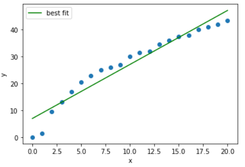
14.4.10. Plot and Best Fit

Compute the least-squares best fit to predict yield based on process temperature. Show the best fit line overlaid on a scatter plot of the data.

# INSTRUCTIONS: The commented out code below has been copied 
# from the farm example. Modify it to use with the new data set.

## fit coefficients 
# b1_, b0_, r_value, p_value, std_err = stats.linregress(x, y)
# print("slope = ",b1_,"pounds per acre / pH unit")
# print("intercept =",b0_,"pounds per acre")


## generate predictions
# pH_pred = np.linspace(4.5, 6.1, 20)
# yld_pred = b0_ + b1_ * pH_pred


## create plot
# plt.plot(pH,yld,'.b',markersize=20,label='Data')
# plt.plot(pH_pred,yld_pred,'-r',linewidth=3,label='Best Fit Line')
# plt.xlabel('Soil pH')
# plt.ylabel('Dry Matter Yield [pounds / acre]')
# plt.grid(True)
# plt.legend()
# plt.show()

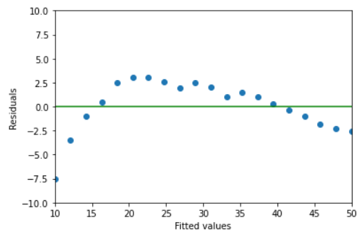
14.4.11. Reisdual Analysis: Part 1

Plot the residuals versus the fitted values. Does the linear model seem appropriate? Write a sentence to explain.

# INSTRUCTIONS: The commented out code below has been copied 
# from the farm example. Modify it to use with the new data set.

## calculate residuals
# yld_hat = b0_ + b1_ * pH
# e_farm = yld - yld_hat
# print("Residuals (pounds / acre):")
# print(e_farm)


## create plot
# plt.plot(yld_hat,e_farm,"b.",markersize=20)
# plt.xlabel("Predicted Yield (pounds / acre)")
# plt.ylabel("Residual (pounds / acre)")
# plt.grid(True)
# plt.show()

14.4.12. Residual Analysis: Part 2

Plot the residuals versus the data collection order. Is there a trend in the residuals with time? Does the linear model seem appropriate?

## create plot