8.2. Electricity Market Optimization#
Home Activity
You are expected to read this entire notebook before class.
8.2.1. Learning Objectives#
After studying this notebook, completing the activities, and asking questions in class, you should be able to:
Solve more complex optimization problems using pyomo.
Create mathematical models on paper.
Answer questions using/interpreting the pyomo model results.
'''
This cell installs Pyomo and Ipopt on Google Colab. To run this notebook
locally (e.g., with anaconda), you first need to install Pyomo and Ipopt.
'''

import sys
if "google.colab" in sys.modules:
    !wget "https://raw.githubusercontent.com/ndcbe/CBE60499/main/notebooks/helper.py"
    import helper
    helper.install_idaes()
    helper.install_ipopt()
import numpy as np
import matplotlib.pyplot as plt
import pandas as pd
from pyomo.environ import *
8.2.2. Optimal Operation of Battery Energy Storage#
Grid-scale battery energy storage systems (BESS) are expected to play a critical role in supporting wide-spread adoption of renewable electricity. In an effort to future proof their electric grid, California has mandated over 1 GW of BESS power capacity be brought online by 2020. For context, the peak electricity demand in California for 2021 was 44 GW.
For policy-makers, technology developers, and investors, there is a critical need to understand the true value of energy storage systems. In California and many regions throughout the United States, electricity is purchased and sold in a wholesale market with time-varying prices (units of $ / MWh). In principle, a smart battery operator wants to buy low (charge) and sell high (discharge). This is known as energy arbitrage.
8.2.3. Visualize Price Data#
The text file Prices_DAM_ALTA2G_7_B1.csv contains an entire year of wholesale energy prices for Chino, CA. Let’s import and inspect the data using Pandas. Our text file contains only one column and no header. We will manually specify “Price” as the name for the single column.
Class Activity
Run the code below.
data = pd.read_csv('https://raw.githubusercontent.com/ndcbe/data-and-computing/main/notebooks/data/Prices_DAM_ALTA2G_7_B1.csv',names=['Price'])
data.head()
| Price | |
|---|---|
| 0 | 36.757 |
| 1 | 34.924 |
| 2 | 33.389 |
| 3 | 32.035 |
| 4 | 33.694 |
Let’s compute some summary statistics.
data.describe()
| Price | |
|---|---|
| count | 8760.000000 |
| mean | 32.516994 |
| std | 9.723477 |
| min | -2.128700 |
| 25% | 26.510000 |
| 50% | 30.797500 |
| 75% | 37.544750 |
| max | 116.340000 |
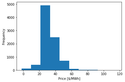
Let’s make a histogram.
plt.hist(data['Price'])
plt.xlabel("Price [$/MWh]")
plt.ylabel("Frequency")
plt.show()
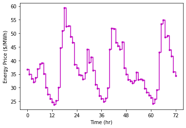
Finally, let’s plot the prices for the first three days in the data set.
# determine number of hours to plot
nT = 3*24

# determine hour we should start counting
# 0 means start counting at the first hour, i.e., midnight on January 1, 2015
t = 0 + np.arange(nT+1)
price_data = data["Price"][t]

# Make plot.
plt.figure()
plt.step(t,price_data,'m.-',where='post')
plt.xlabel('Time (hr)')
plt.ylabel('Energy Price ($/MWh)')
plt.xticks(range(0,nT+1,12))
plt.show()
8.2.4. Create Mathematical Model#
For simplicity, assume a battery energy storage system is price-taker, i.e., they are subject to the market price but their actions do not influence the market price. During each hour \(t\), the battery operator decided to either charge (buy energy) or discharge (sell energy) at rates \(c_t\) and \(d_t\) (units: MW), respectively, subject to the market price \(p_t\) (units: $/MWh).
Assume the battery has a round trip efficiency of \(\eta = 88\%\). Let \(E_t\) represent the state-of-charge at time \(t\) (units: MW).
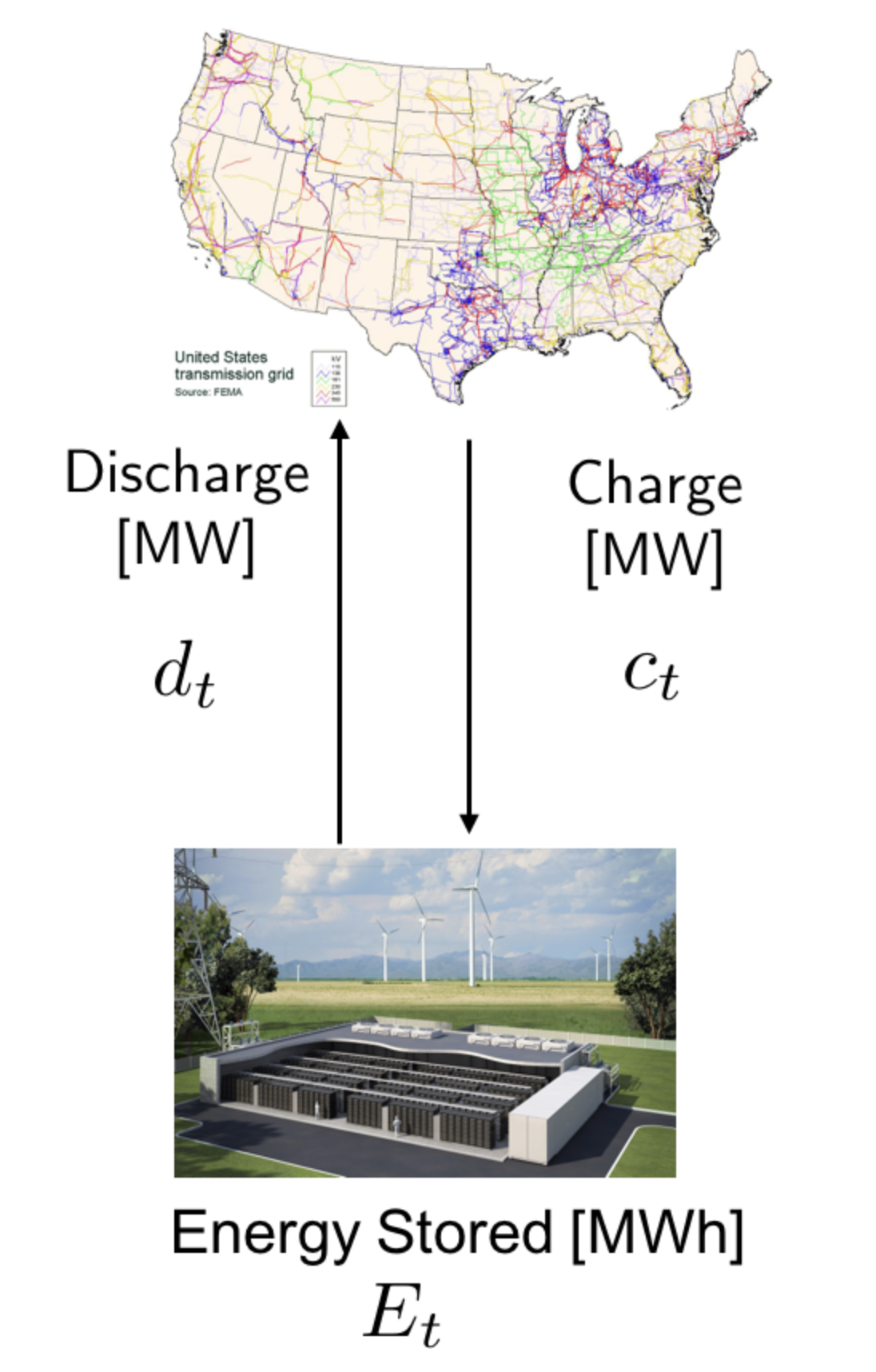
Class Activity
Using the picture above, sketch the battery system. Label \(d_t\), \(c_t\), \(E_t\), and \(p_t\) on your sketch. Verify the units are consistent.
We can now write a constrained optimization problem to compute the optimal market participation strategy (when to buy and sell).
Class Activity
Discuss the optimization problem above with a partner. Then, write a few sentences to explain each equation.
8.2.5. Define Pyomo Model#
We can now write the optimization problem in Pyomo. We will create a set TIME to write the model compactly. For a review on creating concrete models, refer to the previous notebook (01-Pyomo-Basics).
Class Activity
Finish the Pyomo model below.
# define a function to build model
def build_model(price,e0 = 0):
    '''
    Create optimization model for battery operation

    Inputs:
        price: Pandas DataFrame with energy price timeseries
        e0: initial value for energy storage level

    Output:
        model: Pyomo optimization model
    '''

    # Create a concrete Pyomo model.
    model = ConcreteModel()

    ## Define Sets

    # Number of timesteps in planning horizon
    model.TIME = Set(initialize = price.index)

    ## Define Parameters

    # Square root of round trip efficiency
    model.sqrteta = Param(initialize = sqrt(0.88))

    # Energy in battery at t=0
    model.E0 = Param(initialize = e0, mutable=True)

    # Charging rate [MW]
    model.c = Var(model.TIME, initialize = 0.0, bounds=(0, 1))

    # Add your solution here

    ## Define constraints

    # Define Energy Balance constraints. [MWh] = [MW]*[1 hr]
    # Note: this model assumes 1-hour timestep in price data and control actions.
    def EnergyBalance(model,t):
        # First timestep
        if t == 0 :
            return model.E[t] == model.E0 + model.c[t]*model.sqrteta-model.d[t]/model.sqrteta

        # Subsequent timesteps
        else :
            # Add your solution here

    model.EnergyBalance_Con = Constraint(model.TIME, rule = EnergyBalance)

    ## Define the objective function (profit)
    # Receding horizon
    def objfun(model):
        return  sum((-model.c[t] + model.d[t]) * price[t] for t in model.TIME)
    model.OBJ = Objective(rule = objfun, sense = maximize)

    return model
8.2.6. Solve Optimization Model#
We can now create an instance of our Pyomo model. Notice the function build_model requires we pass in a Pandas DataFrame with the price data. Let’s try the first day only.
# Build the model
instance = build_model(data["Price"][0:24],0.0)

# Specify the solver
solver = SolverFactory('ipopt')

# Solve the model
results = solver.solve(instance, tee = True)
Ipopt 3.11.1:

******************************************************************************
This program contains Ipopt, a library for large-scale nonlinear optimization.
 Ipopt is released as open source code under the Eclipse Public License (EPL).
         For more information visit http://projects.coin-or.org/Ipopt
******************************************************************************

NOTE: You are using Ipopt by default with the MUMPS linear solver.
      Other linear solvers might be more efficient (see Ipopt documentation).


This is Ipopt version 3.11.1, running with linear solver mumps.

Number of nonzeros in equality constraint Jacobian...:       95
Number of nonzeros in inequality constraint Jacobian.:        0
Number of nonzeros in Lagrangian Hessian.............:        0

Total number of variables............................:       72
                     variables with only lower bounds:        0
                variables with lower and upper bounds:       72
                     variables with only upper bounds:        0
Total number of equality constraints.................:       24
Total number of inequality constraints...............:        0
        inequality constraints with only lower bounds:        0
   inequality constraints with lower and upper bounds:        0
        inequality constraints with only upper bounds:        0

iter    objective    inf_pr   inf_du lg(mu)  ||d||  lg(rg) alpha_du alpha_pr  ls
   0 2.1094237e-015 1.13e-002 2.99e+001  -1.0 0.00e+000    -  0.00e+000 0.00e+000   0
   1 -1.4124684e-001 1.07e-002 2.72e+001  -1.0 2.03e-001    -  8.78e-002 4.88e-002f  1
   2 -2.6373063e+000 8.29e-003 2.74e+001  -1.0 8.21e-001    -  5.78e-002 2.27e-001f  1
   3 -2.2360880e+001 6.20e-003 2.78e+001  -1.0 3.20e+000    -  3.56e-002 2.52e-001f  1
   4 -3.8049600e+001 5.73e-003 2.51e+001  -1.0 8.23e+000    -  9.39e-002 7.63e-002f  1
   5 -5.9077018e+001 4.87e-003 2.34e+001  -1.0 6.97e+000    -  8.18e-002 1.50e-001f  1
   6 -7.9367583e+001 3.64e-003 2.18e+001  -1.0 4.22e+000    -  9.20e-002 2.52e-001f  1
   7 -8.5414120e+001 3.02e-003 1.71e+001  -1.0 2.06e+000    -  2.10e-001 1.72e-001f  1
   8 -8.9903789e+001 1.64e-003 1.17e+001  -1.0 1.23e+000    -  3.29e-001 4.57e-001f  1
   9 -9.2816651e+001 9.05e-004 3.65e+000  -1.0 1.25e+000    -  6.67e-001 4.48e-001f  1
iter    objective    inf_pr   inf_du lg(mu)  ||d||  lg(rg) alpha_du alpha_pr  ls
  10 -9.3848256e+001 4.09e-004 1.17e+000  -1.0 9.08e-001    -  6.61e-001 5.48e-001f  1
  11 -9.3998203e+001 3.54e-005 6.77e-002  -1.0 7.33e-001    -  1.00e+000 9.13e-001f  1
  12 -9.8037848e+001 4.44e-016 2.55e-003  -1.7 1.37e-001    -  9.88e-001 1.00e+000f  1
  13 -9.9097566e+001 4.44e-016 9.77e-015  -2.5 5.13e-002    -  1.00e+000 1.00e+000f  1
  14 -9.9251854e+001 4.44e-016 2.64e-003  -3.8 2.84e-002    -  9.49e-001 1.00e+000f  1
  15 -9.9252231e+001 4.44e-016 7.61e-015  -3.8 6.38e-004    -  1.00e+000 1.00e+000f  1
  16 -9.9260699e+001 4.44e-016 1.02e-014  -5.7 6.12e-004    -  1.00e+000 1.00e+000f  1
  17 -9.9260804e+001 4.44e-016 1.55e-005  -8.6 8.42e-006    -  1.00e+000 9.97e-001f  1
  18 -9.9260804e+001 8.88e-016 2.84e-001  -8.6 2.56e-008    -  8.71e-001 1.00e+000f  1
  19 -9.9260804e+001 8.88e-016 7.58e-015  -8.6 2.64e-009    -  1.00e+000 1.00e+000h  1

Number of Iterations....: 19

                                   (scaled)                 (unscaled)
Objective...............: -9.9260804110396435e+001  -9.9260804110396435e+001
Dual infeasibility......:  7.5766950348697468e-015   7.5766950348697468e-015
Constraint violation....:  8.8817841970012523e-016   8.8817841970012523e-016
Complementarity.........:  3.0241425605247924e-009   3.0241425605247924e-009
Overall NLP error.......:  3.0241425605247924e-009   3.0241425605247924e-009


Number of objective function evaluations             = 20
Number of objective gradient evaluations             = 20
Number of equality constraint evaluations            = 20
Number of inequality constraint evaluations          = 0
Number of equality constraint Jacobian evaluations   = 20
Number of inequality constraint Jacobian evaluations = 0
Number of Lagrangian Hessian evaluations             = 19
Total CPU secs in IPOPT (w/o function evaluations)   =      0.056
Total CPU secs in NLP function evaluations           =      0.000

EXIT: Optimal Solution Found.
8.2.7. Extract Solution from Pyomo#
Excellent. Ipopt terminated with the message Optimal Solution Found. Let’s inspect the answer.
Class Activity
Run the code below.
# Declare empty lists
c_control = []
d_control = []
E_control = []
time = []

# Loop over elements of TIME set.
for i in instance.TIME:
    # Record the time
    time.append(value(i))

    # Use value( ) function to extract the solution for each variable and append to the results lists
    c_control.append(value(instance.c[i]))

    # Adding negative sign to discharge for plotting
    d_control.append(-value(instance.d[i]))
    E_control.append(value(instance.E[i]))
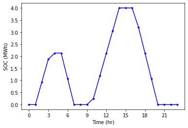
8.2.8. Plot Results#
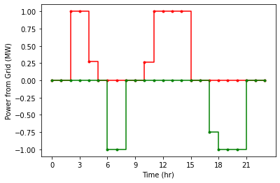
Now let’s plot the optimal charge and discharge profile.
# Plot the state of charge (E)
plt.figure()
plt.plot(time,E_control,'b.-')
plt.xlabel('Time (hr)')
plt.ylabel('SOC (MWh)')
plt.xticks(range(0,24,3))
plt.show()

# Plot the charging and discharging rates
# we can do a step/stair plot as the control values are constant across each hr
plt.figure()
plt.step(time,c_control,'r.-',where="post")
plt.step(time,d_control,'g.-',where="post")
plt.xlabel('Time (hr)')
plt.ylabel('Power from Grid (MW)')
plt.xticks(range(0,24,3))
plt.show()
8.2.9. How much money can a 4 MWh battery make in a year?#
Class Activity
Copy the code from the cell below the heading Solve Optimization Model to the cell below. Then modify to calculate the revenue for an entire year. Hint: Do NOT modify the function create_model.
# Add your solution here