Problem Set 1

CBE 60258, University of Notre Dame. © Prof. Alexander Dowling, 2023

You may not distribution homework solutions without written permissions from Prof. Alexander Dowling.

# Load required Python libraries.
# Please do not remove or rename anything in this cell. The autograder
# assumes numpy is loaded as 'np'
import numpy as np
import scipy
from scipy import linalg
import matplotlib.pyplot as plt

1. Air Conditioner

Learning Objectives: In this problem, you’ll practice solving a mass balance problem with linear algebra (and Python). We’ll then explore how a specific modeling mistake causes our solution approach to fail… and why this makes sense based on linear algebra. This is a fun problem. Past (undergraduate) students said this was their “ah ha!” moment when they saw the connection between three classes: linear alegbra, introduction to chemical engineering, and numerical and statistical analysis. This is an old exam problem, extended to include Python for the homework.

You want to determine the operating conditions of an air conditioning unit. The feed into the air conditioning unit is moist air, and the output is liquid water and somewhat drier air. It is relatively easy to measure the mole fraction of the air and water in each stream, but measuring the flow rates of the streams is a lot harder. If we know the composition of the streams, we can compute the flow rates via component and overall mass balances.

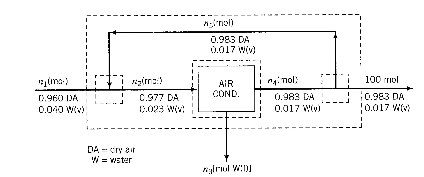
Caption: Flowsheet for an air conditioning unit (simplified). Variables \(n_1\), …, \(n_5\) are (unknown) molar flows. Mole fractions are given for each stream (DA is dry air, W is water). From Felder and Rousseau (2005).

1a. Mathematical Model

Propose a system of linearly independent equations that relate \(n_1\), \(n_2\), \(n_3\), \(n_4\), and \(n_5\). Label your equations, such as “overall mass balance around entire system”. Finally, write your model in matrix form. Turn in your handwritten work via Gradescope.

1b. Numerical Solution

Solve for \(n_1\) through \(n_5\) in Python. Store your answer in the numpy array n_flow in order from \(n_1\) to \(n_5\).

# Add your solution here

# Print solutions. Note the use of the .format() function, which provides a convenient way
# to display messages on screen.
print('The molar flows are:')
for i in range(len(n_flow)):
    print("n{0} = {1:0.3f} mol".format(i+1,n_flow[i]))

The autograder will check your answer stored in n_flow.

# Removed autograder test. You may delete this cell.

1c. Diagnostics

Your classmate attempts to model the system as:

\[\begin{split} \begin{equation} \begin{bmatrix} 1 & 0 & -1 & 0 & 0 \\ 0 & 1 & -1 & -1 & 0 \\ 0 & 0.977 & 0 & -0.983 & 0 \\ 0 & 0.023 & -1 & -0.017 & 0 \\ 0 & 0 & 0 & 1 & -1 \\ \end{bmatrix} \cdot \begin{bmatrix} n_1 \\ n_2 \\ n_3 \\ n_4 \\ n_5 \end{bmatrix} = \begin{bmatrix} 100 \\ 0 \\ 0 \\ 0 \\ 100 \end{bmatrix} \end{equation} \end{split}\]

but their Python code is not working. Your classmate says, “I am not sure about the mass balances around the air conditioner.”

Answer the questions below. Hint: Flow \(n_3\) is pure liquid water.

Q1: What is the rank and condition number of the \(A\) matrix in your classmate’s model?

(You may calculate rank with Python using numpy.linalg.matrix_rank and numpy.linalg.cond. Please either print out the answers to the screen.)

# Please take a minute to verify this matrix matches
# the A matrix in your classmate's model.
A = np.array([[1, 0, -1, 0, 0],[0, 1, -1, -1, 0],[0, 0.977, 0, -0.983, 0],
              [0, 0.023, -1, -0.017, 0],[0, 0, 0, 1, -1]])
print("A=\n",A)

# Add your solution here

Q2: What is wrong with the model? How are the rank and condition number helpful in answering this question?

Q3: What mistake did your classmate make?

Q4: How can you fix the model?

Your Answer:

2. Estimating Thermal Gradient with Three Probes

We have previously considered the optimal depth of a temperature probe in a metal slab to estimate the thermal gradient. Please take a few minutes to review that material. You will turn in your written work for this problem via Gradescope.

Your boss now wants to use three probes to reduce the error in estimating the temperature gradient. Let’s see if they are right.

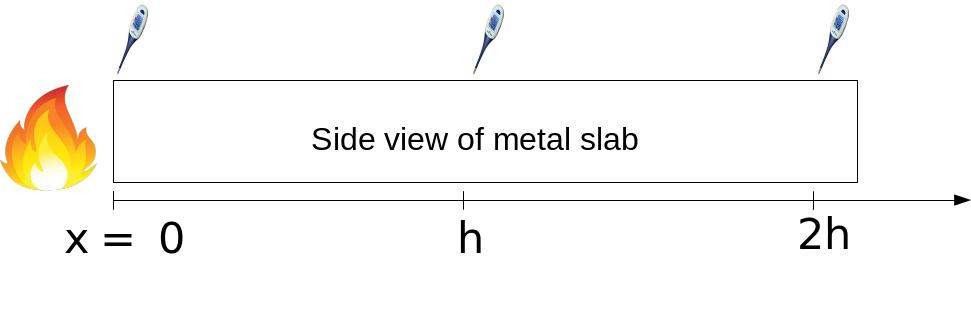
Assumption 1: Probe 1 is placed at \(x=0\), probe 2 is placed at \(x=h\), and probe 3 is placed at \(x=2h\).

Assumption 2: The temperature profile in the slab given by the equation:

(1)\[\begin{equation} T = T_0 - \alpha e^{\beta x} \end{equation}\]

where \(\alpha\) = 2 °C and \(\beta\) = 0.5 cm\(^{-1}\). The probes have a random error (\( \sigma_T \)) of \(\pm\)0.1 °C.

Assumption 3: The random errors in the temperature measurements are independent.

2a. Taylor Series for Three Probe System

Recall, the temperature measured by the 2 probe system was written out as a Taylor series expansion:

(2)\[\begin{equation} \left. T \right|_{x=1h} = \left. T \right|_{x=0} + (1h) \left. \frac{\partial T}{\partial x} \right|_{x=0} + \frac{1}{2!} (1h)^2 \left. \frac{\partial^2 T}{\partial x^2} \right|_{x = l} \end{equation}\]

Using this as a reference, write the Taylor series expansion (up to the first four terms) for \(T\) at \(x=h\) and \(x=2h\).

Submit your answer and written work via Gradescope.

2b. Finite Difference Formula

Using your answer from 2a, write the finite difference formula for the three probe system.

Hint: Eliminate the quadratic term from the Taylor series expansion to give an expression that looks like:

(3)\[\begin{equation} \left. \frac{\partial{T}}{\partial{x}} \right|_{x=0} = \frac{\boxed{?} \ T(0) + \boxed{?} \ T(h) + \boxed{?} \ T(2h)}{h} + \boxed{?} \end{equation}\]

where you determine the expressions to replace \(\boxed{?}\).

Submit your answer and written work via Gradescope.

2c. Algorithm Error

Determine the algorithm error for estimating \(\frac{\partial{T}}{\partial{x}}\) at \(x = 0\).

Submit your answer and written work via Gradescope.

2d. Random Error

Determine the random error for estimating \(\frac{\partial{T}}{\partial{x}}\) at \(x = 0\).

Hint: Use the addition error propagation formula given by:

(4)\[\begin{equation} \sigma_z^2 = \left(c_1^2 + c_2^2 + c_3^2\right)\sigma_T^2 \end{equation}\]

Submit your answer and written work via Gradescope.

2e. Optimal Location

What is the optimum value of \(h\) for which the error in measuring the temperature gradient is minimum? What is the minimum error?

Submit your answer and written work via Gradescope.

3. Finite Difference Approximations

Main Idea: Explore the accuracy of the finite difference approximation for \(\nabla f(x)\) and \(\nabla^2 f(x)\) (matricies of first and second derivatives).

## Load libraries
from mpl_toolkits.mplot3d import Axes3D
from matplotlib import cm
import sympy as sym
# from sympy import symbols, diff

3a. Finite difference order

Repeat the analysis from class to show the backward and central finite difference truncations errors are \(\mathcal{O}(\epsilon)\) and \(\mathcal{O}(\epsilon^2)\), respectively. We discussed these error orders graphically. Please use a Taylor series for your analysis.

Test Problem

Consider the function

\[\begin{split} \begin{align*} f(\mathbf{x}) &= \alpha \mathrm{exp}(-\beta) \\ u &= x_1 - 0.8 \\ v &= x_2 - (a_1 + a_2 u^2 \sqrt{1 - u} - a_3 u) \\ \alpha &= -b_1 + b_2 u^2 \sqrt{1 - u} + b_3 u \\ \beta &= c_1 v^2 (1 - c_2 v) / (1 + c_3 u^2) \\ {\mathbf{a}} &= [0.3, 0.6, 0.2]^T \\ {\mathbf{b}} &= [5, 26, 3]^T \\ {\mathbf{c}} &= [40, 1, 10]^T \end{align*} \end{split}\]

This is Example 2.19 in Biegler (2010). For our purposes, it is a complicated function we do not want to analytically differentiate.

Provided Codes

Please review the following code. You do not need to turn anything in for this section.

Finite Difference Code

The code below has been adapted from the finite difference examples presented in class. Notice the second input is a function.

## Define Python function
def my_f(x,verbose=False):
    ''' Evaluate function given above at point x

    Inputs:
        x - vector with 2 elements
        
    Outputs:
        f - function value (scalar)
    '''
    # Constants
    a = np.array([0.3, 0.6, 0.2])
    b = np.array([5, 26, 3])
    c = np.array([40, 1, 10])
    
    # Intermediates. Recall Python indicies start at 0
    u = x[0] - 0.8
    s = np.sqrt(1-u)
    s2 = np.sqrt(1+u)
    v = x[1] -(a[0] + a[1]*u**2*s-a[2]*u)
    alpha = -b[0] + b[1]*u**2*s2+ b[2]*u 
    beta = c[0]*v**2*(1-c[1]*v)/(1+c[2]*u**2)
    
    if verbose:
        print("##### my_f at x = ",x, "#####")
        print("u = ",u)
        print("sqrt(1-u) = ",s)
        print("sqrt(1+u) = ",s2)
        print("v = ",v)
        print("alpha = ",alpha)
        print("beta = ",beta)
        print("f(x) = ",)
        print("##### Done. #####\n")
    
    return alpha*np.exp(-beta)

## Calculate gradient with central finite difference
def my_grad_approx(x,f,eps1,verbose=False):
    '''
    Calculate gradient of function my_f using central difference formula
    
    Inputs:
        x - point for which to evaluate gradient
        f - function to consider
        eps1 - perturbation size
        
    Outputs:
        grad - gradient (vector)
    '''
    
    n = len(x)
    grad = np.zeros(n)
    
    if(verbose):
        print("***** my_grad_approx at x = ",x,"*****")
    
    for i in range(0,n):
        
        # Create vector of zeros except eps in position i
        e = np.zeros(n)
        e[i] = eps1
        
        # Finite difference formula
        my_f_plus = f(x + e)
        my_f_minus = f(x - e)
        
        # Diagnostics
        if(verbose):
            print("e[",i,"] = ",e)
            print("f(x + e[",i,"]) = ",my_f_plus)
            print("f(x - e[",i,"]) = ",my_f_minus)
        
        
        grad[i] = (my_f_plus - my_f_minus)/(2*eps1)
    
    if(verbose):
        print("***** Done. ***** \n")
    
    return grad

## Calculate gradient using central finite difference and my_hes_approx
def my_hes_approx(x,grad,eps2):
    '''
    Calculate gradient of function my_f using central difference formula and my_grad
    
    Inputs:
        x - point for which to evaluate gradient
        grad - function to calculate the gradient
        eps2 - perturbation size (for Hessian NOT gradient approximation)
        
    Outputs:
        H - Hessian (matrix)
    '''
    
    n = len(x)
    H = np.zeros([n,n])
    
    for i in range(0,n):
        # Create vector of zeros except eps in position i
        e = np.zeros(n)
        e[i] = eps2
        
        # Evaluate gradient twice
        grad_plus = grad(x + e)
        grad_minus = grad(x - e)
        
        # Notice we are building the Hessian by column (or row)
        H[:,i] = (grad_plus - grad_minus)/(2*eps2)

    return H

### Test the functions from above

## Define test point
xt = np.array([0,0])
print("xt = ",xt,"\n")

print("f(xt) = \n",my_f([0,0]),"\n")

## Compute gradient
g = my_grad_approx(xt,my_f,1E-6)
print("grad(xt) = ",g,"\n")

## Compute Hessian
# Step 1: Create a Lambda (anonymous) function
calc_grad = lambda x : my_grad_approx(x,my_f,1E-6)

# Step 2: Calculate Hessian approximation
H = my_hes_approx(xt,calc_grad,1E-6)
print("hes(xt) = \n",H,"\n")

Analytic Gradient

It turns out that calculating the analytic gradient with Mathematic quickly becomes a mess. Instead, the following code uses the symbolic computing capabilities in SymPy.

'''
Encoding the exact gradient with the long expression above is very time-consuming. This is a trick of calculating the 
symbolic derivative and converting it to an analytic function to be evaluated at a point. 
'''

# Define function to use with symbolic computing framework
def f(x1,x2):
    a = np.array([0.3, 0.6, 0.2])
    b = np.array([5, 26, 3])
    b1 = 5;
    c = np.array([40, 1, 10])
    u = x1 - 0.8
    v = x2 -(a[0] + a[1]*u**2*(1-u)**0.5-a[2]*u)
    alpha = b[1]*u**2*(1+u)**0.5 + b[2]*u -b[0]
    beta = c[0]*v**2*(1-c[1]*v)/(1+c[2]*u**2)
    return alpha*sym.exp(-1*beta)

# Define function to use later
def my_grad_exact(x):
    x1, x2 = sym.symbols('x1 x2')
    DerivativeOfF1 = sym.lambdify((x1,x2),sym.diff(f(x1,x2),x1));
    DerivativeOfF2 = sym.lambdify((x1,x2),sym.diff(f(x1,x2),x2));
    #DerivativeOfF2 = sym.lambdify((x1,x2),gradf2(x1,x2));
    #F = sym.lambdify((x1,x2),f(x1,x2));
    return np.array([DerivativeOfF1(x[0],x[1]),DerivativeOfF2(x[0],x[1])])
    
x = np.array([0,0])
print("The exact gradient is \n",my_grad_exact(x))

Analytic Hessian

The code below assembles the analytic Hessian using the symbolic computing framework in NumPy.

def f(x1,x2):
    
    a = np.array([0.3, 0.6, 0.2])
    b = np.array([5, 26, 3])
    b1 = 5;
    c = np.array([40, 1, 10])
    u = x1 - 0.8
    v = x2 -(a[0] + a[1]*u**2*(1-u)**0.5-a[2]*u)
    alpha = b[1]*u**2*(1+u)**0.5 + b[2]*u -b[0]
    beta = c[0]*v**2*(1-c[1]*v)/(1+c[2]*u**2)
    return alpha*sym.exp(-1*beta)


def my_hes_exact(x):
    x1, x2 = sym.symbols('x1 x2')
    HessianOfF11 = sym.lambdify((x1,x2),sym.diff(f(x1,x2),x1,x1));
    HessianOfF12 = sym.lambdify((x1,x2),sym.diff(f(x1,x2),x1,x2));
    HessianOfF21 = sym.lambdify((x1,x2),sym.diff(f(x1,x2),x2,x1));
    HessianOfF22 = sym.lambdify((x1,x2),sym.diff(f(x1,x2),x2,x2));
    #DerivativeOfF2 = sym.lambdify((x1,x2),gradf2(x1,x2));
    #F = sym.lambdify((x1,x2),f(x1,x2));
    return np.array([[HessianOfF11(x[0],x[1]),HessianOfF12(x[0],x[1])],[HessianOfF21(x[0],x[1]),HessianOfF22(x[0],x[1])]])
    
x = np.array([0,0])
print("The exact Hessian is \n",my_hes_exact(x))    

Gradient Finite Difference Comparison

Repeat the analysis procedure from the finite difference class notebook to find the value of \(\epsilon_1\) that gives the smallest approximation error. Some tips:

1. Write a for loop to iterate over many values of \(\epsilon_1\)

2. Use \(|| \nabla f(x;\epsilon_1)_{approx} - \nabla f(x)_{exact} ||\) to measure the error. Your choice on which norm(s) to use. Please label your plot with the norm(s) you used.

3. Make a log-log plot

# Add your solution here

Hessian Finite Difference using Approximate Gradient

Repeat the analysis from above. Use my_grad_approx and the best value for \(\epsilon_1\) you previously found. What value of \(\epsilon_2\) gives the lowest Hessian approximation error? Note: \(\epsilon_1\) is used in the gradient approximation and \(\epsilon_2\) is used in the Hessian approximation.

# Add your solution here

Hessian Finite Difference using Exact Gradient

Repeat the analysis from above using my_grad_exact. What value of \(\epsilon_2\) gives the lower Hessian approximation error?

# Add your solution here

3b. Final Answers

Record your final answers below:

A. Using \(\epsilon_1 = \) … gives error \(|| \nabla f(x;\epsilon_1)_{approx} - \nabla f(x)_{exact} || = \) …

B. Using \(\epsilon_1 = \) … and \(\epsilon_2 = \) … gives error \(|| \nabla^2 f(x;\epsilon_1,\epsilon_2)_{approx} - \nabla^2 f(x)_{exact} || = \) …

C. Using \(\epsilon_2 = \) gives error \(|| \nabla^2 f(x;\epsilon_2)_{approx} - \nabla^2 f(x)_{exact} || = \) …

These answers were computed using the (fill in blank) norm.

What is the benefit of using the exact gradient when approximating the Hessian with central finite difference?

Answer:

4. Multivariable Taylor Series

You will use my_grad_exact, my_grad_approx, my_hes_exact, and my_hes_approx to construct Taylor series approximations to an arbitrary twice differentiable continuous functions with inputs \(x \in \mathbb{R}^2\). We will then consider visualize the Taylor series approximation in 3D.

4a. Create a function to plot the first order Taylor series using \(\nabla f\)

Create a general function that:

1. Constructs a Taylor series using \(\nabla f\) centered around a given point

2. Plots the true function and Taylor series approximation

def taylor1(xc, f, grad, dx):
    '''
    Constructs a Taylor series using first derivates and visualizes in 3D
    
    Arguments:
        xc - point to center Taylor series
        f - function that computes function value. Only has one input (x)
        grad - function that computes gradient. Only has one input (x)
        dx - list or numpy array. creates 3D plot over xc[0] +/- dx[0], xc[1] +/- dx[1]
    
    Returns:
        none
        
    Actions:
        3D plot
    
    '''
    
    # Add your solution here

First order Taylor Series using my_grad_approx

Consider \(x_c = [0.7, 0.3]^T\) (center of Taylor series) and \(\Delta x = [0.5, 0.5]^T\) (domain for plot).

# Specify epsilon1
calc_grad = lambda x : my_grad_approx(x,my_f,1E-6)

# Specify dx
dx = [0.5, 0.5]

# Specify xc
xc = np.array([0.7, 0.3])

taylor1(xc, my_f, calc_grad, dx)

First order Taylor Series using my_grad_exact

Consider \(x_c = [0.7, 0.3]^T\) (center of Taylor series) and \(\Delta x = [0.5, 0.5]^T\) (domain for plot).

# Specify epsilon1
calc_grad = lambda x : my_grad_exact(x)

# Specify dx
dx = [0.5, 0.5]

# Specify xc
xc = np.array([0.7, 0.3])

taylor1(xc, my_f, calc_grad, dx)

Create a function to plot the second order Taylor series using \(\nabla f\) and \(\nabla^2 f\)

def taylor2(xc, f, grad, hes, dx):
    '''
    Constructs a Taylor series using first derivates and visualizes in 3D
    
    Inputs:
        xc - point to center Taylor series
        f - computes function value. Only has one input (x)
        grad - computes gradient. Only has one input (x)
        hes - computes the Hessian. Only has one input (x)
        dx - creates 3D plot over xc[0] +/- dx[0], xc[1] +/- dx[1]
    
    Outputs:
        none
        
    Creates:
        3D plot
    
    '''
    
    ### Evaluates function and gradiant
    fval = f(xc)
    gval = grad(xc)
    Hval = hes(xc)
    
    ### Creates domain for plotting
    x1 = np.arange(xc[0] - dx[0],xc[0] + dx[0],dx[0]/100)
    x2 = np.arange(xc[1] - dx[1],xc[1] + dx[1],dx[1]/100)
    
    ## Create a matrix of all points to sample
    X1, X2 = np.meshgrid(x1, x2)
    n1 = len(x1)
    n2 = len(x2)

    ## Allocate matrix for true function value
    F = np.zeros([n2, n1])

    ## Allocate matrix for Taylor series approximation
    T = np.zeros([n2, n1])    
    
    xtemp = np.zeros(2)

    # Evaluate f(x) and Taylor series over grid
    for i in range(0,n1):
        xtemp[0] = x1[i]
        for j in range(0,n2):
            xtemp[1] = x2[j]
            
            # Evaluate f(x)
            F[j,i] = my_f(xtemp)

            # Evaluate Taylor series
            dx_ = xtemp - xc
            
            '''
            print("dx = ",dx)
            print("gval = ",gval)
            print("Hval = ",Hval)
            '''
            
            temp = Hval.dot(dx_)
            # print("Hval * dx = ",temp)
            
            
            # T[j,i] = fval + gval.dot(dx_) + 0.5*(temp).dot(dx_)
            T[j,i] = fval + gval.dot(dx_) + 0.5*(dx_.dot(Hval.dot(dx_)))
            
    # Create 3D figure
    fig = plt.figure()
    ax = fig.gca(projection='3d')

    # Plot f(x)
    surf = ax.plot_surface(X1, X2, F, linewidth=0,cmap=cm.coolwarm,antialiased=True,label="f(x)")

    # Plot Taylor series approximation
    surf = ax.plot_surface(X1, X2, T, linewidth=0,cmap=cm.PiYG,antialiased=True,label="Taylor series")
    
    # Add candidate point
    ax.scatter(xc[0],xc[1],fval,s=50,color="black",depthshade=True)

    # Draw vertical line through stationary point to help visualization
    # Maximum value in array
    fmax = np.amax(F)
    fmin = np.amin(F)
    ax.plot([xc[0], xc[0]], [xc[1], xc[1]], [fmin,fmax],color="black")
    
    plt.show()

Second order Taylor series using my_grad_approx and my_hes_approx

Consider \(x_c = [0.7, 0.3]^T\) (center of Taylor series) and \(\Delta x = [0.2, 0.2]^T\) (domain for plot).

# Specify epsilon1
calc_grad = lambda x : my_grad_approx(x,my_f,1E-6)

# Specify epsilon2
calc_hes = lambda x : my_hes_approx(x, calc_grad, 1E-6)

# Specify dx
dx = [0.2, 0.2]

# Specify xc
xc = np.array([0.7, 0.3])

taylor2(xc, my_f, calc_grad, calc_hes, dx)

Second order Taylor series using my_grad_exact and my_hes_exact

Consider \(x_c = [0.7, 0.3]^T\) (center of Taylor series) and \(\Delta x = [0.2, 0.2]^T\) (domain for plot).

x = np.array([0,0])
# Specify epsilon1
calc_grad = lambda x : my_grad_exact(x)

# Specify epsilon2
calc_hes = lambda x1 : my_hes_exact(x1)

# Specify dx
dx = [0.2, 0.2]

# Specify xc
xc = np.array([0.7, 0.3])

taylor2(xc, my_f, calc_grad, calc_hes, dx)

4b. Discussion

Write 1 or 2 sentences to describe the the shapes for the first order and second order Taylor series approximations? Why do these shapes make sense?

Answer:

Is there a visible difference in the Taylor series approximations using the finite difference versus exact derivatives? Why does this make sense?

Answer: