8.3. Flash Calculations in Pyomo#
Home Activity
You are expected to read this entire notebook before class.
8.3.1. Learning Objectives#
After studying this notebook, completing the activities, and asking questions in class, you should be able to:
Apply the process of creating a mathematical model and implementing it in pyomo to any nonlinear optimization problem.
Understand and interpret the solutions to a pyomo model.
'''
This cell installs Pyomo and Ipopt on Google Colab. To run this notebook
locally (e.g., with anaconda), you first need to install Pyomo and Ipopt.
'''

import sys
if "google.colab" in sys.modules:
    !wget "https://raw.githubusercontent.com/ndcbe/CBE60499/main/notebooks/helper.py"
    import helper
    helper.install_idaes()
    helper.install_ipopt()
import numpy as np
import matplotlib.pyplot as plt
import pandas as pd
from pyomo.environ import *
8.3.2. Flash Example Revisited#
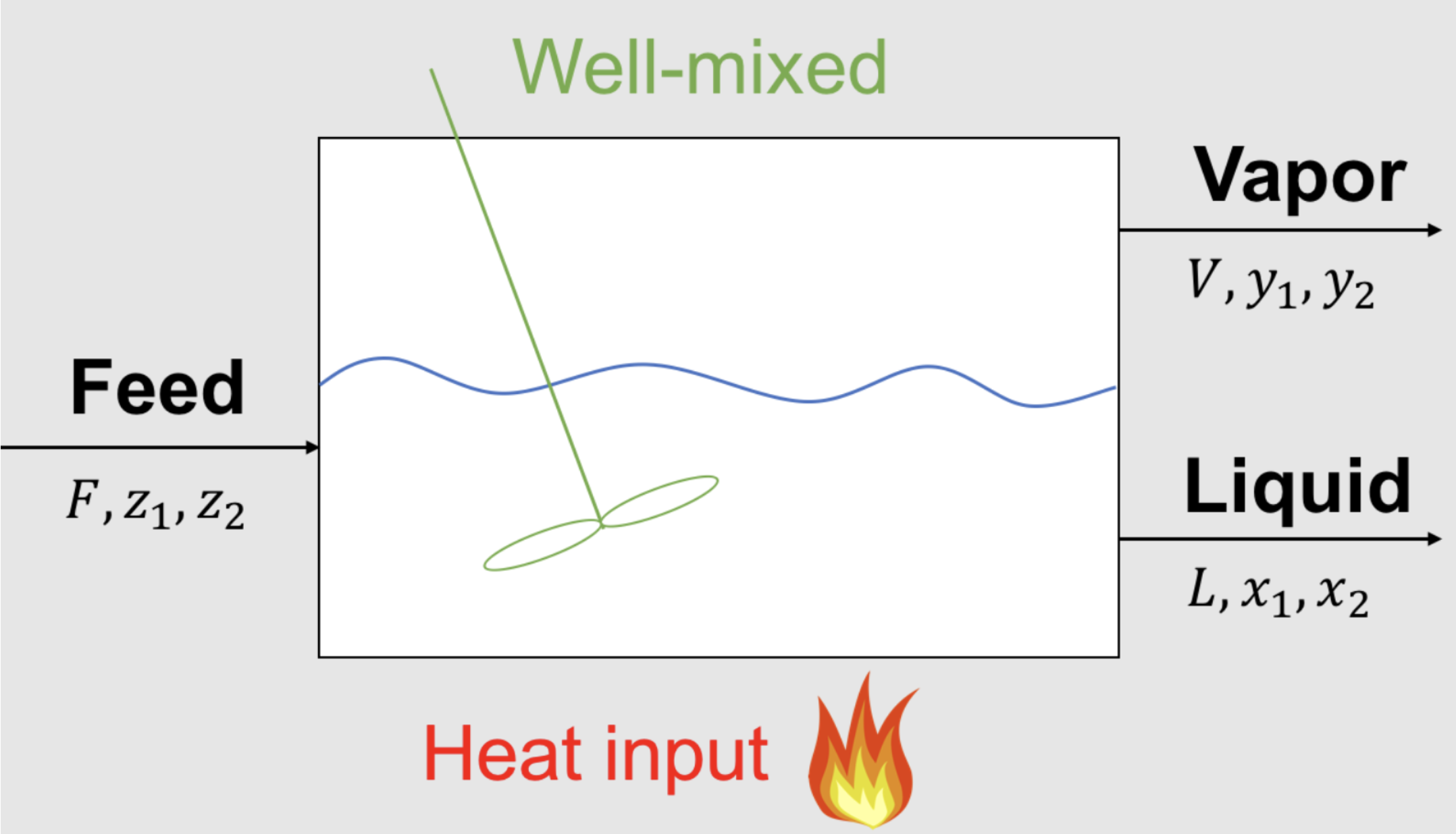
Let’s revist the flash example from this previous notebook. Here is the mathematical model:
Feed Specifications: \(F = 1.0\) mol/s, \(z_1\) = 0.5 mol/mol, \(z_2\) = 0.5 mol/mol
Given Equilibrium Data: \(K_1\) = 3 mol/mol, \(K_2\) = 0.05 mol/mol
Overall Material Balance:
Component Mass Balances:
Thermodynamic Equilibrium:
Summation:
And here is part of the code from this previous Newton’s Method notebook:
def my_f(x):
    ''' Nonlinear system of equations in canonical form F(x) = 0
    Copied from Lecture 7.

    Arg:
        x: vector of variables

    Returns:
        r: residual, F(x)

    '''

    # Initialize residuals
    r = np.zeros(6)

    # given data
    F = 1.0
    z1 = 0.5
    z2 = 0.5
    K1 = 3
    K2 = 0.05

    # copy values from x to more meaningful names
    L = x[0]
    V = x[1]
    x1 = x[2]
    x2 = x[3]
    y1 = x[4]
    y2 = x[5]

    # equation 1: overall mass balance
    r[0] = V + L - F

    # equations 2 and 3: component mass balances
    r[1] = V*y1 + L*x1 - F*z1
    r[2] = V*y2 + L*x2 - F*z2

    # equation 4 and 5: equilibrium
    r[3] = y1 - K1*x1
    r[4] = y2 - K2*x2

    # equation 6: summation
    r[5] = (y1 + y2) - (x1 + x2)
    # This is known as the Rachford-Rice formulation for the summation constraint

    return r
Class Activity
Complete the pyomo model below using the code above and solve the flash calculation.
## Create a concrete model
m = ConcreteModel()

## Define the objective to be a constant
m.obj = Objective(expr=1)

## Define a set for components
m.COMPS = Set(initialize=[1,2])

## given data
m.F = Param(initialize=1.0)
m.z = Param(m.COMPS, initialize={1:0.5, 2:0.5})

# Add your solution here

## Define variables
m.L = Var(initialize=0.5)
m.V = Var(initialize=0.5)
m.x = Var(m.COMPS, bounds=(0, 1.0), initialize={1:0.5, 2:0.5})
# Add your solution here

### Define equations

# equation 1: overall mass balance
m.overall_mass_balance = Constraint(expr=m.F == m.V + m.L)

# equations 2 and 3: component mass balances
def eq_comp_mass_balance(model, c):
    ''' model: Pyomo model
        c: set for components
    '''

    return model.V * model.y[c] + model.L * model.x[c] == model.F * model.z[c]

m.component_mass_balance = Constraint(m.COMPS, rule=eq_comp_mass_balance)

# equation 4 and 5: equilibrium
# Add your solution here

# equation 6: summation
# Add your solution here
# This is known as the Rachford-Rice formulation for the summation constraint

## Print model
m.pprint()
## Solve the model

# Specify the solver
solver = SolverFactory('ipopt')

# Solve!
results = solver.solve(m, tee = True)
## Examine the solution
print("L = ",value(m.L),"mol/s")
# Add your solution here