12.6. Monte Carlo Error Propagation#
12.6.1. Learning Objectives#
After studying this notebook, completing the activities, engaging in class, and reading the book, you should be able to:
Understand and apply Monte Carlo error propogation
import numpy as np
import matplotlib.pyplot as plt
In this notebook we will take the motivating car and incline example from this notebook a step further to apply Monte Carlo Error Propogation.
12.6.2. Analytic Error Propagation for Student 1#
## Results of 'standard' error analysis (from homework)

# define distance travelled
l = 1 # m

# define function to calculate a1
calc_a1 = lambda v: v**2 / (2*l)

# define velocity measurement and uncertainty
v = 3.2
v_std = 0.1

# calculate a1
a1 = calc_a1(v)

# estimate gradient with forward finite difference
da1dv = (calc_a1(v + 1E-6) - a1)/(1E-6)

# calculate uncertainty
sigma_a1 = abs(da1dv)*v_std

# report answer
print("Calculated acceleration: ",round(a1,2),"+/-",round(sigma_a1,2),"m/s/s")
Calculated acceleration: 5.12 +/- 0.32 m/s/s
12.6.3. Monte Carlo Error Propagation for Student 1#
We can also estimate the uncertainty in \(a_1\) using simulation. See more about simulation in this notebook. Below is the main idea.
Repeat 1000s of times:
Add \(\mathcal{N}(0,0.1^2)\) uncertainty to velocity measurement
Recalculate \(a_1\) and store result
Then calculate the standard deviation of the stored \(a_1\) results. In other words, we are simulated what would happen if we repeated the experiment many many times with an assumed random measurement error.
Class Activity
With a partner, complete the code below.
# specify number of simulations
nsim = 1000

# create vector to store the results
a1_sim = np.zeros(nsim)

# Add your solution here

# create histogram of calculated a1 values
plt.hist(a1_sim)
plt.xlabel("Acceleration (m/s/s)")
plt.ylabel("Number of Simulations")
plt.show()

# print some descriptive statistics
print("Mean: ",np.mean(a1_sim)," m/s/s")
print("Median: ",np.median(a1_sim)," m/s/s")
print("Standard Deviation: ",np.std(a1_sim)," m/s/s")
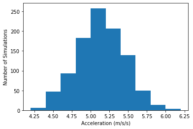
Mean:  5.132195705031086  m/s/s
Median:  5.123636307619483  m/s/s
Standard Deviation:  0.3177820622012161  m/s/s
This standard deviation matches the uncertainty calculated with the error propagation formulas.
12.6.4. Analytic Error Propagation for Student 2#
## Results of 'standard' error analysis (from homework)

# define distance travelled
l = 1 # m

# define function to calculate a2
calc_a2 = lambda t: 2*l / t**2

# define time measurement and uncertainty
t = 0.63
t_std = 0.01

# calculate a2
a2 = calc_a2(t)

# estimate gradient with forward finite difference
da2dt = (calc_a2(t + 1E-6) - a2)/(1E-6)

# calculate uncertainty
sigma_a2 = abs(da2dt)*t_std

print("Calculated acceleration: ",round(a2,2),"+/-",round(sigma_a2,2),"m/s/s")
Calculated acceleration: 5.04 +/- 0.16 m/s/s
12.6.5. Monte Carlo Error Propagation for Student 2#
Class Activity
Apply the Monte Carlo approach to Student 2’s calculation. Start by copying and pasting the code from above.
# Add your solution here
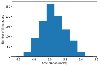
Mean:  5.047666385956689  m/s/s
Median:  5.039586271630645  m/s/s
Standard Deviation:  0.15621555703632722  m/s/s