13.8. Statistical Power Basics#

Reference: §6.13 and §6.13 in Navidi (2015).

# load libraries
import scipy.stats as stats
from scipy.stats import norm
import numpy as np
import math
import matplotlib.pyplot as plt

13.8.1. Learning Objectives#

After studying this notebook, completing the activities, participating in class, and reviewing your notes, should be able to:

Compute statistical power.
Explain the significance of the statistical power calculation.

13.8.2. Definition#

The power of a statistical test, \(1-\beta\), is the probability of rejecting \(H_0\) given \(H_a\) is true:

\[ \mathrm{power} = 1 - \beta = \mathbb{P}\left(~\mathrm{reject}~H_0 ~~|~~ H_a~\mathrm{is~true}~\right) \]

In other words, statistical power measures our ability to detect something new (alternate hypothesis) within background uncertainty. Several factors impact statistical power:

The statistical significance level \(\alpha\)
Magnitude of the effect of interest in the population
Sample size

Statistical power calculations should be done before gathering data. They help inform experiment design.

Home Activity

A test has power 0.9 when \(\mu = 15\). Determine if each statement below is true or false. Store your answer in the Python dictionary tf_18c using 1, 2, 3, and 4 as the key.

Statements:

The probability of rejecting \(H_0\) when \(\mu = 15\) is 0.90.
The probability of making a correct decision when \(\mu = 15\) is 0.90.
The probability of making a correct decision when \(\mu = 15\) is 0.10.
The probability that \(H_0\) is true when \(\mu = 15\) is 0.10.

# Declare dictionary. You need to change each entry to True or False.
# Do not use 'True' or 'False', but instead True or False
tf_18c = {}
tf_18c[1] = 'change me'
tf_18c[2] = 'change me'
tf_18c[3] = 'change me'
tf_18c[4] = 'change me'

# Add your solution here

# Removed autograder test. You may delete this cell.

13.8.3. Motivating Example#

We want to test if a new chemical manufacturing process has a high yield than the current process. Based on years of historical data, we know the current process has a mean yield 80 and standard deviation 5. The units for yield are percentage of the theoretical maximum. We drop the “%” symbol for clarity.

Our supervisor proposed to run the new process 50 times and then perform hypothesis testing using significance level \(\alpha\) = 0.05:

\[H_0: \mu \leq 80 \qquad \mathrm{versus} \qquad H_a: \mu > 80\]

where \(\mu\) is the mean yield of the new process. But running 50 tests is expensive. Eyeing a new promotion, you want to know if it is reasonable to run only 20 or 30 experiments. You need to perform a statistical power calculation. We will walk through the steps now.

13.8.4. Step 1. Fix the experiment design, make assumptions.#

More specifically, we need to:

Fix the number of experiments, for example \(n\) = 50
Fix the significance level, for example \(\alpha\) = 0.05
Assume the mean for the new process yield, for example \(\mu\) = 81 (a modest improvement in yield)
Assume the standard deviation for the new process yield, for example \(\sigma\) = 5 (same as old process)

# number of trials
n = 50

# significance level
alpha = 0.05

# assumed mean and standard deviation for new process (alternate distribution)
mu = 81
s = 5

# mean and standard deviation for current process (null distribution)
mu0 = 80
s0 = 5

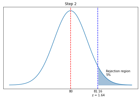
13.8.5. Step 2. Compute the rejection region.#

We want to calculate the sample mean (yield averaged over the \(n\) = 50 runs) threshold that corresponds with the specified significance level \(\alpha = 0.05\). Because we have such a large sample size, we will use the normal distribution (z-test) for simplicity.

# This function is the inverse cdf for a normal distribution.
# We give it the probability and it gives the corresponding z value.
z = stats.norm.ppf(1-alpha)
print(z)

1.6448536269514722

Thus we will reject the null hypothesis for set of 50 runs where the \(z > 1.1645\). We will call this the rejection region.

# Significant level(α)
alpha = 0.05
# Critical value for α
crit_val = norm.ppf(1-alpha)
x = np.linspace(norm.ppf(0.0001),norm.ppf(0.9999), 100)
plt.figure(figsize=(8,5))
plt.plot(x, norm.pdf(x))
plt.fill_between(x[x>crit_val], 0, norm.pdf(x)[x>crit_val].flatten(),alpha=0.5, color='steelblue')
plt.axvline(x=crit_val,color='b',linestyle='dashed')
plt.axvline(x=0,color='r',linestyle='dashed')
plt.text(crit_val-0.35, -.06, 'z = 1.64'.format(round(crit_val,2), str(alpha)), fontsize=10)
plt.text(crit_val-0.25, -.04, '81.16'.format(round(crit_val,2), str(alpha)), fontsize=10)
plt.text(0-.1, -.04, '80'.format(round(crit_val,2), str(alpha)), fontsize=10)
plt.text(crit_val+0.5, 0.05, 'Rejection region\n5%', fontsize=10)
plt.title('Step 2')
ax = plt.gca()
plt.xticks([])
plt.yticks([])
plt.show()

../../_images/Statistical-Power-Basics_14_0.png

We can go a step further and express this \(z\) cutoff in terms of the sample mean. Recall,

\[ z = \frac{\bar{X}_{rr} - \mu_0}{\sigma_0/\sqrt{n}} \]

A little algebra, and

\[ \bar{X}_{rr} = z \frac{\sigma_0}{\sqrt{n}} + \mu_0 \]

rr = z*s0/math.sqrt(n) + mu0
print(rr)

81.16308715367667

Thus we reject the null hypothesis when \(\bar{X} > 81.16\).

13.8.6. Step 3. Compute the statistical power.#

We will now construct the alternate distribution with mean \(\mu\) and standard deviation \(\sigma/\sqrt{n}\). Recall, we assumed values for \(\mu\) and \(\sigma\) in Step 1. We will then calculate the probability of drawing a sample mean from the alternate distribution that is in the rejection region.

# Significant level(α)
alpha = 0.05
# Critical value for α
crit_val = norm.ppf(1-alpha)
new_crit = crit_val-1
x = np.linspace(norm.ppf(0.0001),norm.ppf(0.9999), 100)
plt.figure(figsize=(8,5))
plt.plot(x, norm.pdf(x), x, norm.pdf(x+1))
plt.fill_between(x[x>new_crit], 0, norm.pdf(x)[x>new_crit].flatten(),alpha=0.5, color='steelblue')
plt.axvline(x=new_crit,color='b',linestyle='dashed')
plt.axvline(x=0,color='r',linestyle='dashed')
plt.text(.3, -.07, 'z = 1.64'.format(round(crit_val,2), str(alpha)), fontsize=10)
plt.text(.4, -.05, '81.16'.format(round(crit_val,2), str(alpha)), fontsize=10)
plt.text(0-.1, -.05, '81'.format(round(crit_val,2), str(alpha)), fontsize=10)
plt.text(-1.1, -.05, '80'.format(round(crit_val,2), str(alpha)), fontsize=10)
plt.text(crit_val+0.5, 0.05, 'Power = 0.4090', fontsize=10)
plt.text(-3.5, 0.25, 'Null Distribution', fontsize=10)
plt.text(1.1, 0.25, 'Alternate Distribution', fontsize=10)

plt.title('Step 3')
ax = plt.gca()
plt.xticks([-1,0,new_crit])
ax.set_xticklabels([])
plt.yticks([])
plt.show()

../../_images/Statistical-Power-Basics_19_0.png

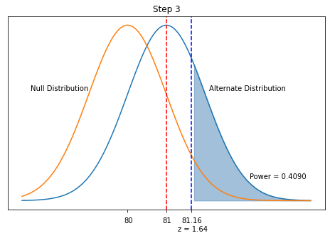
We want to calculate, under the assumed alternate distribution, the probably of drawing a sample mean that is in the rejection zone. This is the shaded area in the figure above.

\[ z_1 = \frac{\bar{X}_{rr} - \mu}{\sigma / \sqrt{n}} \]

\[ \mathrm{power} = \mathbb{Pr}[Z \geq z_1], \qquad Z \sim \mathcal{N}(0,1) \]

z1 = (rr - mu)/(s/math.sqrt(n))
print("z1 =",z1)
print("power =",1 - stats.norm.cdf(z1))

z1 = 0.23064006457837258
power = 0.4087972197938724

Interpretation Even with 50 experiments, there is only a 40.9% chance we will reject the null hypothesis and conclude the new process is better. Remember, the calculated statistical power depends on \(n\), \(\alpha\), \(\mu\) and \(\sigma\) (assumptions).

Home Activity

Based on this analysis, your team concludes that improving yield from 80 to 81 percent of theoretical maximum performance is not worth the capital investment. Upper management will only approve the new process if it has a mean yield of at least 84 percent. Copy the code for above to answer the following two questions.

13.8.7. Activity: Question 1#

What is the statistical power with \(n=50\) if we assume the mean yield of the new process is 84 and same standard deviation of the current process? Store your answer in the Python float ans_18c_i.

# Hint: Copy and paste the code for the three steps above, then modify.

## Step 1

## BEGIN SOLUTION

# number of trials
n = 50

# significance level
alpha = 0.05

# assumed mean and standard deviation for new process (alternate distribution)
mu = 84
s = 5

# mean and standard deviation for current process (null distribution)
mu0 = 80
s0 = 5

## END SOLUTION

## Step 2

# Add your solution here

## Step 3

# Add your solution here

## Store answer (statistical power) in ans_18c_i.

# Add your solution here

81.16308715367667
z1 = -4.012000622540913
power = 0.9999698968293542

# Removed autograder test. You may delete this cell.

13.8.8. Activity: Question 2#

Using the same assumptions, what is the smallest sample size with a statistical power of at least 99.9%?

## Step 1

## BEGIN SOLUTION

# number of trials
n = 35

# significance level
alpha = 0.05

# assumed mean and standard deviation for new process (alternate distribution)
mu = 84
s = 5

# mean and standard deviation for current process (null distribution)
mu0 = 80
s0 = 5

## END SOLUTION

## Step 2

# Add your solution here

## Step 3

# Add your solution here

## Store answer (sample size) in ans_18c_ii.

# Add your solution here

81.39015504122366
z1 = -3.0880101995282256
power = 0.9989924922251623

# Removed autograder test. You may delete this cell.

Home Activity

Write down at least one question how have on statistical power calculations.

Your Questions:

Data and Computing for Chemical Engineers

Statistical Power Basics

Contents

13.8. Statistical Power Basics#

13.8.1. Learning Objectives#

13.8.2. Definition#

13.8.3. Motivating Example#

13.8.4. Step 1. Fix the experiment design, make assumptions.#

13.8.5. Step 2. Compute the rejection region.#

13.8.6. Step 3. Compute the statistical power.#

13.8.7. Activity: Question 1#

13.8.8. Activity: Question 2#