11.4. Normal Probability Distributions

Further Reading: §4.5 in Navidi (2015)

11.4.1. Learning Objectives

After studying this notebook, completing the activities, engaging in class, and reading the book, you should be able to:

• Model scientific and engineering problems using the normal distribution.

• Use standard normal z-table to compute probabilities.

import numpy as np

11.4.2. Definition

The normal distribution (a.k.a. Gaussian) is a good model for many continuous random variables in science and engineering. As we will soon see, the normal distributions is also extremely important in statistics.

Here is the probability density function:

\[ f(x) = \frac{1}{\sigma \sqrt{2 \pi}} e^{-(x-\mu)^2 / (2\sigma^2)} \]

The normal distribution is charactered by two parameters, \(\mu\) and \(\sigma\), which are the mean and standard deviation:

\[ \mu_X = \int_{-\infty}^{\infty} x \frac{1}{\sigma \sqrt{2 \pi}} e^{-(x-\mu)^2 / (2\sigma^2)} dx = \mu \]

\[ \sigma^2_X = \int_{-\infty}^{\infty} (x - \mu_X)^2 \frac{1}{\sigma \sqrt{2 \pi}} e^{-(x-\mu)^2 / (2\sigma^2)} dx = \sigma^2 \]

Navidi (2015) walks through the calculus on pg. 251 and 252.

We write \(X \sim \mathcal{N}(\mu, \sigma^2)\).

11.4.3. 68-95-99.7 Rule

Here is how to draw a normal distribution on paper.

1. Draw a symmetric “bell” curve.

2. Label the peak \(\mu\).

3. Label the points of inflection \(\mu - \sigma\) and \(\mu + \sigma\).

4. \(\sigma\) is the distance between the peak and the points of inflection. Using this distance, label \(\mu \pm 2 \sigma\) and \(\mu \pm 3 \sigma\).

As alluded to a few times this semester, there is not an analytic expression for integrating the normal PDF. Instead, we must use numeric integration. Most engineers, scientists, and statisticians memorize three specific areas under the normal curve, which is called the 68-95-99.7 rule.

\[\int_{\mu - \sigma}^{\mu + \sigma} \frac{1}{\sigma \sqrt{2 \pi}} e^{-(x-\mu)^2 / (2\sigma^2)} dx \approx 0.6827\]

\[\int_{\mu - 2 \sigma}^{\mu + 2 \sigma} \frac{1}{\sigma \sqrt{2 \pi}} e^{-(x-\mu)^2 / (2\sigma^2)} dx \approx 0.9545\]

\[\int_{\mu - 3 \sigma}^{\mu + 3 \sigma} \frac{1}{\sigma \sqrt{2 \pi}} e^{-(x-\mu)^2 / (2\sigma^2)} dx \approx 0.9973\]

11.4.4. Standardization

Let \(X \sim \mathcal{N}(\mu, \sigma^2)\). It is much more convienent to standardize by defining a new variable \(Z\):

\[Z = \frac{X - \mu}{\sigma}\]

Now let’s convert the three integrals for the 68-95-99.7 rule from \(x\) to \(z\). First, let’s solve for \(x\).

\[z = \frac{x - \mu}{\sigma} \rightarrow x = z \sigma + \mu\]

Recall the normal PDF:

\[f(x) = \frac{1}{\sigma \sqrt{2 \pi}} e^{-(x-\mu)^2 / (2\sigma^2)}\]

Now substitute:

\[f(z) = \frac{1}{\sigma \sqrt{2 \pi}} e^{-(z\sigma + \mu -\mu)^2 / (2\sigma^2)}\]

And simplify:

\[f(z) = \frac{1}{\sigma \sqrt{2 \pi}} e^{-z^2 / 2}\]

Now let’s transform the limits of integration:

\[x = \mu + c \sigma\]

Now substitute:

\[z \sigma + \mu = \mu + c \sigma\]

And simplify:

\[z = c\]

Now let’s transform the \(dx\) into a \(dz\). First we differentiate:

\[\sigma dz = dx\]

And then subsitutite:

\[\int_{\mu - c \sigma}^{\mu + c \sigma} \frac{1}{\sigma \sqrt{2 \pi}} e^{-(x-\mu)^2 / (2\sigma^2)} dx = \int_{-c}^{c} \frac{1}{\sqrt{2 \pi}} e^{-z^2 / 2} dz\]

We see that \(Z\) follows a normal distribution with mean 0 and variance 1, i.e., \(Z \sim \mathcal{N}(0, 1)\). This is known as a standard normal distribution.

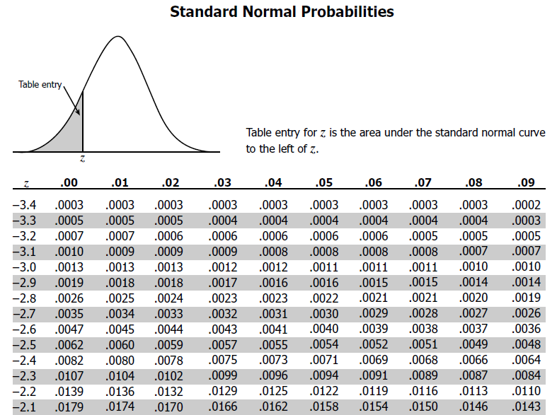
The front cover of your textbook has precomputed the cumulative distribution function for the standard normal. This is known as a z-table.

11.4.5. Example: Using the Z-Table

Class Activity

Use the Z-table to answer the following questions.

As an intern at Frozen Pizza, Inc. you learn the fat content of single serving pies is normally distributed with mean 10g with standard deviation 0.2 g.

What is the probability the next pizza coming off the manufacturing line has more than 10.4 grams of fat?

Answer:

The FDA would like you to certify that 99% of frozen pizzas have fat content between ______ and ______ grams, where the interval in centered at the mean. Fill in the blanks.

Blank 1:

Blank 2:

11.4.6. Example: Modeling Stocks

Let’s say we want to predict the outcome of the stock market next year. We create a simple model using a normal distribution with mean 1.5% return and standard deviation 4.5% return.

According to our model, is the probability we will lose money next year if we invest in the stock market?

Class Activity

Work through the example below together.

11.4.7. Approach 1: Numerically integrate the pdf

from scipy import integrate
def normal_pdf(x,mean,stdev):
    '''PDF for normal distribution
    Arg:
        x: outcome value
        mean: mean
        stdev: standard deviation
    
    Return: probability    
    '''
    
    assert stdev > 0.0
    
    var = stdev**2
    
    return (1/np.sqrt(2*np.pi*var)) * np.exp(-(x - mean)**2 / 2 / var)

# Integrate numerically. We'll learn the details of how this works later in the class.

my_f = lambda x: normal_pdf(x, mean=1.5, stdev=4.5)

integrate.quad(my_f,-10000,0)

(0.36944134018176356, 5.073409550679581e-12)

11.4.8. Approach 2: Standardize and use function for standard normal distribution

z = (0 - 1.5) / 4.5
print(z)

-0.3333333333333333

from scipy import stats
stats.norm.cdf(z)

0.36944134018176367