14.7. Multivariate Linear Regression#
14.7.1. Learning Objectives#
After studying this notebook and your lecture notes, you should be able to:
Fit multivariate models (including polynomials) using linear regression
Using the 538 blog post as an example, explain why claiming a trend line is “statistically significant” can be misleading or not informative
# load libraries
import scipy.stats as stats
import numpy as np
import scipy.optimize as optimize
import math
import matplotlib.pyplot as plt
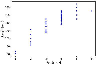
14.7.2. Motivating Example: Predict Bluegills Age#
Data source: https://newonlinecourses.science.psu.edu/stat501/node/325/
# age of fish in years
age = np.array([1,1,2,2,2,2,3,3,3,3,3,3,3,3,3,2,3,4,4,4,4,4,4,4,4,4,4,4,4,4,4,4,
                4,4,4,4,4,5,4,4,4,5,2,2,4,3,4,3,4,4,4,4,3,3,3,4,4,3,4,5,4,5,4,4,
                3,5,5,4,5,3,4,3,4,6,4,5,4,4])

# length of fish in mm
length = np.array([67,62,109,83,91,88,137,131,122,122,118,115,131,143,142,123,122,
                   138,135,146,146,145,145,144,140,150,152,157,155,153,154,158,162,
                   161,162,165,171,171,162,169,167,188,100,109,150,140,170,150,140,
                   140,150,150,140,150,150,150,160,140,150,170,150,150,150,150,150,
                   150,160,140,160,130,160,130,170,170,160,180,160,170])

plt.plot(age,length,'b.')
plt.xlabel("Age [years]")
plt.ylabel("Length [mm]")
plt.show()

Can we use the age of the fish to predict its length?
14.7.3. Normal Equations#
Recall from 12-02 and 12-03 the formulation for multivariate linear regression:
Observations: \(\vec{y} = [y_1, y_2, ..., x_n]^T\)
Fitted Parameters: \(\vec{\beta} = [\beta_0, \beta_1, ..., \beta_{m}]^T\)
Data / Feature Matrix:
For example, we could fit a linear model where reactor yield depended on both temperature, pressure and inlet compositions.
The linear regression best fit estimates can be easily computed with linear algebra:
or
where the \(\vec{~}\) is omitted for simplicity. Above are know as the normal equations.
By applying the error propagation formula to the above equation, we can easily calculate the covariance matrix of the fitted parameters:
14.7.4. Attempt 1. Linear Model#
Let’s start with a simple regression model:
where \(x_1\) is the length of the fish.
Class Activity
Construct the feature matrix X.
nfish = len(age)

# feature matrix (store in 'X')
# Add your solution here

print("X =\n",X)
Class Activity
Compute \((\mathbf{X}^T \mathbf{X})^{-1}\) and store in XXinv.
# calculate inverse of XT * X
# Add your solution here
print("inv(XT X) =\n",XXinv)
Class Activity
Compute \(\hat{\mathbf{\beta}}\) (fitted coefficients) and store in beta_hat.
# recall we can calculate the best fit coefficients with linear algebra
# Add your solution here
print("beta_hat =",beta_hat)
Class Activity
Complete the code below to evaluate the model and plot the predictions.
## evaluate predictions

# create ages to evaluate model with
age_plot = np.linspace(1,6,100)

# create new X matrix with 100 rows and 2 columns
Xplot = np.ones((len(age_plot),2))

# fill in second column
# Add your solution here

# evaluate model and store in `length_plot`
# Add your solution here

# plot
plt.plot(age,length,'b.',markersize=10,label="Data")
plt.plot(age_plot,length_plot,'r-',label="Best Fit")
plt.xlabel("Age [years]")
plt.ylabel("Length [mm]")
plt.legend()
plt.show()
Class Activity
Calculate and plot the residuals.
# calculate residuals, store in `e`
# Add your solution here

plt.plot(age,e,'b.')
plt.xlabel("Age [years]")
plt.ylabel("Residuals [mm]")
plt.show()
Class Activity
Compute the variance of the residuals. Then compute the covariance of the fitted parameters.
# compute variance of residuals, store in `se`
# Add your solution here
print("variance of residuals = ",se,"add units")

# compute covariance matrix, store in `Sigma_beta`
# Add your solution here
print("covariance matrix:\n",Sigma_beta)
14.7.5. Attempt 2. Quadratic Model#
Let’s try a quadratic model now:
where \(x_1\) is the age and \(x_2\) is age squared.
Class Activity
With a partner, modify the code below (copied from previous example) to and fit the quadratic model.
# construct the feature matrix
X = np.ones((nfish,3))

# Add your solution here

print("X =\n",X)
# calculate inverse of XT * X, store in XXinv
# Add your solution here
print("inv(XT X) =\n",XXinv)
# recall we can calculate the best fit coefficients with linear algebra, store in beta_hat
# Add your solution here
print("beta_hat =",beta_hat)
## evaluate predictions

# create ages to evaluate model with
age_plot = np.linspace(1,6,100)

# create new X matrix with 100 rows and 2 columns
Xplot = np.ones((len(age_plot),3))

# fill in second and third column
# Add your solution here

# evaluate model, store predictions in length_plot
# Add your solution here

# plot
plt.plot(age,length,'b.',markersize=10,label="Data")
plt.plot(age_plot,length_plot,'r-',label="Best Fit")
plt.xlabel("Age [years]")
plt.ylabel("Length [mm]")
plt.legend()
plt.show()
# calculate residuals, store in `e`
# Add your solution here

plt.plot(age,e,'b.')
plt.xlabel("Age [years]")
plt.ylabel("Residuals [mm]")
plt.show()
# compute the variance of residuals, store in `e`
# Add your solution here


# compute covariance matrix, store in `Sigma_beta`
# Add your solution here
print("covariance matrix:\n",Sigma_beta)
14.7.6. How to select the best model?#
We can calculate a p-value to determine if a model is statistically significant.
https://fivethirtyeight.com/features/science-isnt-broken/#part1

