6.6. Newton Methods in Scipy#
6.6.1. Learning Objectives#
After studying this notebook, completing the activities, and asking questions in class, you should be able to:
Use numpy to solve the flash example problem from the Newton’s Method for Systems of Equations notebook.
# load libraries
import numpy as np
from scipy import optimize
6.6.2. Using scipy instead#
numpy and scipy offer a few different implementations of Newton’s method. However, we found these to be unreliable in the past. Instead, we recommend either using the Newton solver we put together in the Newton’s Method for Systems of Equations notebook or Pyomo (future notebook).
However, we will show how this is done using scipy.optimize.newton in this notebook.
Note
Note the difference between scipy.optimize.newton and scipy.optimize.fsolve. The first is used to solve scalar-valued functions (functions that return a single value, i.e. the polynomial example below). The second is used to solve vector-valued functions (functions that return a vector of multiple values, i.e. the flash example below).
# documentation for Newton's method in scipy
help(optimize.newton)
6.6.3. Polynomial Example Revisited Using Scipy#
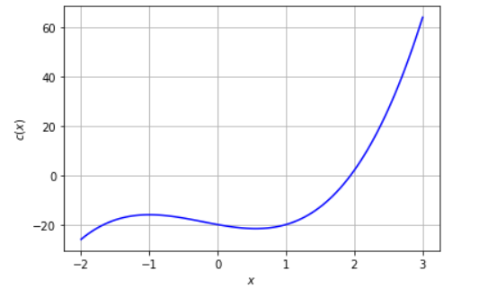
In the following cells we will demonstrate the use of Scipy to perform the Newton-Raphson method for the polynomial example from this previous notebook.
First, we need to run the code we already developed for the polynomial function and its derivative.
def nonlinear_function(x):
    ''' compute a nonlinear function for demonstration
    Arguments:
        x: scalar
    Returns:
        c(x): scalar
    '''
    return 3*x**3 + 2*x**2 - 5*x-20

def Dnonlinear_function(x):
    ''' compute 1st derivative of nonlinear function for demonstration
    Arguments:
        x: scalar
    Returns:
        c'(x): scalar
    '''
    return 9*x**2 + 4*x - 5
Next, we need to provide an initial guess as we did before we the code we deveoped for Newton’s Method.
guess = 1
Now we can run Newton’s Method through scipy.optimize.newton.
polysln = optimize.newton(func=nonlinear_function, x0 = guess, fprime=Dnonlinear_function)
print("The root is found at",polysln)
The root is found at 1.9473052357731322
6.6.4. Flash Problem Revisted Using Scipy#
Recall the flash problem from this previous notebook that we solved in the Newton’s Method for Systems of Equations notebook using Newton’s Method. In the following cells we will demonstrate the use of Scipy to perform the Newton-Raphson method.
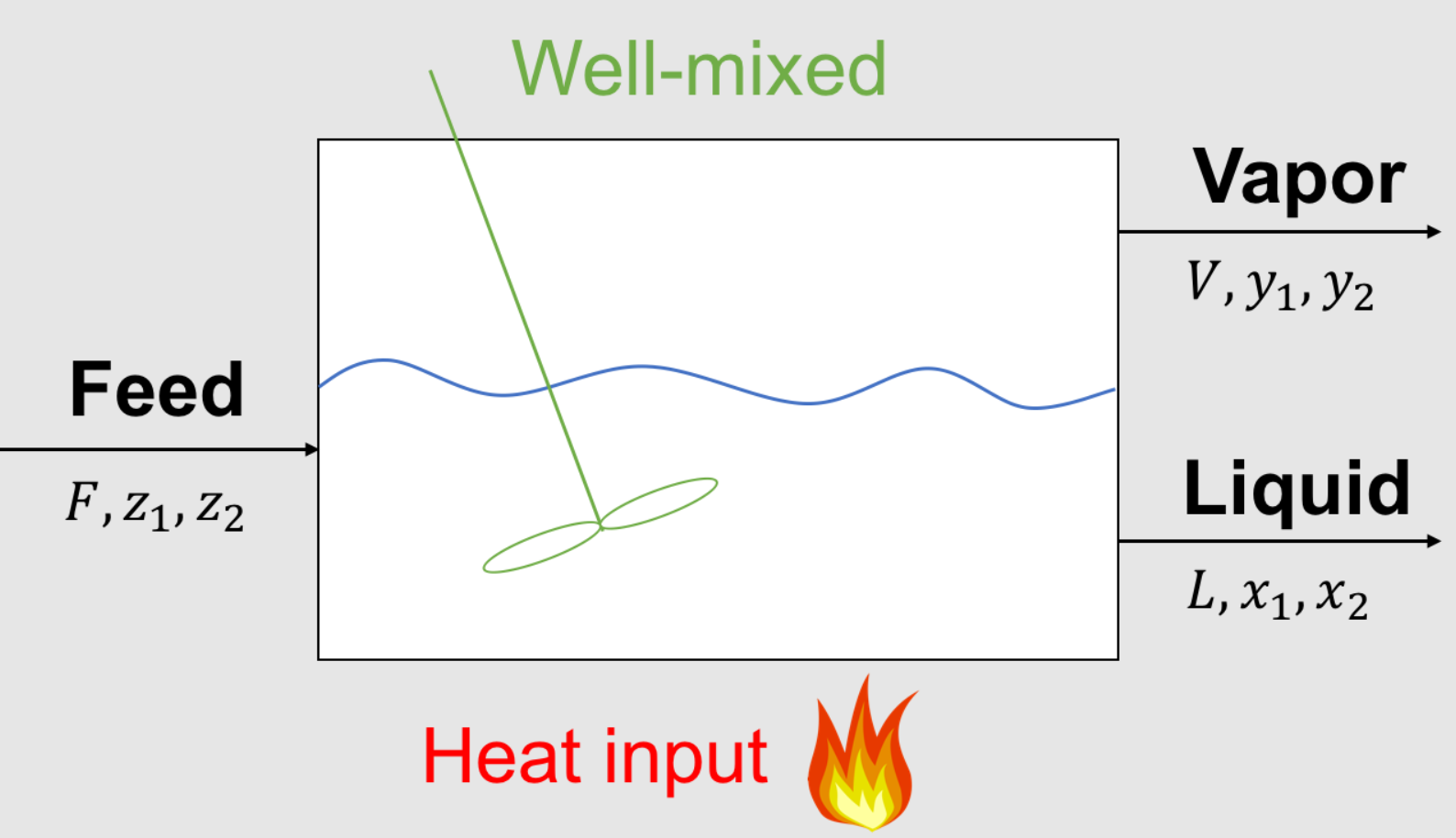
Parameters (given):
\(F\) feed inlet flowrate, mol/time or kg/time
\(z_1\) composition of species 1 in feed, mol% or mass%
\(z_2\) composition of species 2 in feed, mol% or mass%
\(K_1\) partion coefficient for species 1, mol%/mol% or mass% / mass%
\(K_2\) partion coefficient for species 2, mol%/mol% or mass% / mass%
Variables (unknown):
\(L\) liquid outlet flowrate, mol/time or kg/time
\(x_1\) composition of species 1 in liquid, mol% or mass%
\(x_2\) composition of species 2 in liquid, mol% or mass%
\(V\) vapor outlet flowrate, mol/time or kg/time
\(y_1\) composition of species 1 in vapor, mol% or mass%
\(y_2\) composition of species 2 in vapor, mol% or mass%
How to solve the flash problem and other multidimensional problem with \(n\) unknown variables and \(n\) nonlinear equations?
6.6.5. System of Equations in Canonical Form#
with \(\mathbf{x} = (L, V, x_1, x_2, y_1, y_2).\)
First run the code below to define the system of nonlinear equations given in the Newton’s Method for Systems of Equations notebook.
# nonlinear canonical system of equations
def my_f(x,verbose=False):
    ''' Nonlinear system of equations in conancial form F(x) = 0
    Copied from previous notebook.

    Arg:
        x: vector of variables

    Returns:
        r: residual, F(x)

    '''

    # Initialize residuals
    r = np.zeros(6)

    # given data
    F = 1.0
    z1 = 0.5
    z2 = 0.5
    K1 = 3
    K2 = 0.05

    # copy values from x to more meaningful names
    L = x[0]
    V = x[1]
    x1 = x[2]
    x2 = x[3]
    y1 = x[4]
    y2 = x[5]

    # equation 1: overall mass balance
    r[0] = V + L - F

    # equations 2 and 3: component mass balances
    r[1] = V*y1 + L*x1 - F*z1
    r[2] = V*y2 + L*x2 - F*z2

    # equation 4 and 5: equilibrium
    r[3] = y1 - K1*x1
    r[4] = y2 - K2*x2

    # equation 6: summation
    r[5] = (y1 + y2) - (x1 + x2)
    # This is known as the Rachford-Rice formulation for the summation constraint

    if verbose:
        print("Evaluating my_f at x=",x)
        print("Residuals r=",r,"\n")

    return r
6.6.6. Let’s try optimize.newton#
Initially you might be inclined to use optimize.newton as with the polynomial example. Let’s see what happens when we use that below:
# initial guess from the [previous notebook](../04-publish/05-Newton-Raphson-Methods-for-Systems-of-Equations.ipynb).
x0 = np.array([0.5, 0.5, 0.55, 0.45, 0.65, 0.35])
# incorrect scipy function to solve flash example
xsln1 = optimize.newton(func=my_f, x0=x0)
print("Solution using scipy:\n",xsln1)
Solution using scipy:
 [ 5.00004967e-01  5.36467908e-01  1.09276056e+10  3.55480055e+00
 -5.38704523e+36  3.50020142e-01]
C:\Users\ebrea\anaconda3\envs\jbook\lib\site-packages\scipy\optimize\_zeros_py.py:466: RuntimeWarning: some failed to converge after 50 iterations
  warnings.warn(msg, RuntimeWarning)
The correct answer should be [0.72368421 0.27631579 0.3220339 0.6779661 0.96610169 0.03389831]
However, we see that all of the values are incorrect and the third and fifth values diverged.
Consulting the scipy documentation revelas that optimize.newton is only for scalar-valued functions. Notice that optimize.newton did not give a warning about our function being vector-valued; it will not alert you if you use it incorrectly. Instead, it just did not converge.
This illustrates why we choose not to use scipy.optimize.newton for a system of equations. Also, if something does not work as expected, check the documentation.
6.6.7. Instead use optimize.fsolve for multivariate systems#
Instead, we will use optimize.fsolve since this is a vector-valued function (returns a vector of multiple values). We can’t use optimize.newton because it only works for scalar-valued functions (return a single value) like the above polynomial example.
# correct scipy function to solve flash example
xsln = optimize.fsolve(my_f,x0)
print(xsln)
[0.72368421 0.27631579 0.3220339 0.6779661 0.96610169 0.03389831]
6.6.8. Transformed System of Equations in Canonical Form#
One last idea. We can transform the system of equations by introducing the following new log transformed variables for composition:
Now let’s reexamine the equilibrium equations:
Taking the log of both sides of the equations gives:
We then apply properties of logortihms:
And finally substitute the new variables to obtain a new systems of equations:
with \(\mathbf{\bar{x}} = (L, V, \bar{x}_1, \bar{x}_2, \bar{y}_1, \bar{y}_2).\)
# nonlinear canonical system of equations
def my_f_transformed(x_bar,verbose=False):
    ''' Nonlinear system of equations in conancial form F(x) = 0
    Copied from previous notebook.

    Arg:
        x_bar: vector of (partially transformed) variables

    Returns:
        r: residual, F(x)

    '''

    # Initialize residuals
    r = np.zeros(6)

    # given data
    F = 1.0
    z1 = 0.5
    z2 = 0.5
    K1 = 3
    K2 = 0.05

    # copy values from x to more meaningful names
    L = x_bar[0]
    V = x_bar[1]
    log_x1 = x_bar[2]
    log_x2 = x_bar[3]
    log_y1 = x_bar[4]
    log_y2 = x_bar[5]

    # undo transformation (for convience so we do not need to significantly modify the equations below)
    x1 = 10**log_x1
    x2 = 10**log_x2
    y1 = 10**log_y1
    y2 = 10**log_y2

    # equation 1: overall mass balance
    r[0] = V + L - F

    # equations 2 and 3: component mass balances
    r[1] = V*y1 + L*x1 - F*z1
    r[2] = V*y2 + L*x2 - F*z2

    # equation 4 and 5: equilibrium
    r[3] = log_y1 - np.log10(K1) - log_x1
    r[4] = log_y2 - np.log10(K2) - log_x2

    # equation 6: summation
    r[5] = (y1 + y2) - (x1 + x2)
    # This is known as the Rachford-Rice formulation for the summation constraint

    if verbose:
        print("Evaluating my_f_bar at x_bar=",x_bar)
        print("Residuals r=",r,"\n")

    return r
Let’s also define a functon to undo the transformation and print the solution:
Finally, let’s transform the initial guesses from above:
x0_bar = np.array([0.5, 0.5, np.log10(0.55), np.log10(0.45), np.log10(0.65), np.log10(0.35)])
Now, we can try and use optimize.fsovle again with our transformed system.
sln = optimize.fsolve(my_f_transformed,x0_bar)
print(sln)
[ 0.72368421 0.27631579 -0.49209841 -0.16879202 -0.01497716 -1.46982202]
We see that some of the answers are correct, while others are not. From these attempts to find the solution, we have found that it’s best to use the code we develop for Newton’s method or the scipy.optimize.fsolve function.