13.4. Student’s t-Distribution

Further Reading: §5.3 in Navidi (2015)

13.4.1. Learning Objectives

After studying this notebook, attending class, completing the home activities, and asking questions, you should be able to:

• Calculate any size confidence interval (95%, 99%, etc.) using z- or t-distribution

• Explain why the t-distribution is important. Relate this back to the CLT

• Check for the assumption required to apply the t-distribution

# load libraries
import scipy.stats as stats
import numpy as np
import math
import matplotlib.pyplot as plt

13.4.2. Main Idea

What happens if the sample size is small and we do not know \(\sigma\)? Two complications arise:

• Cannot invoke central limit theorem

• Need to account for errors when estimating \(\sigma\) (population standard deviation) using \(s\) (sample standard deviation)

Solution: Student’s t-distribution

History Side Tangent

Published in 1908 by William Sealy Goshet under the pseudonym Student.

13.4.3. Degrees of Freedom and Visualization

\(\nu\) is the degrees of freedom:

• Student’s t-distribution converges to the Gaussian distribution (normal distribution shown in last notebook) as \(\nu \rightarrow \infty\)

• \(\nu\) is often \(n\) - 1. We lose 1 degree of freedom to estimate standard deviation

13.4.4. Comparison of \(z^*\) and \(t^*\)

n = 5
print("Consider n =",n)

# calculate zstar
# argument 1: confidence level
zstar95 = stats.norm.interval(0.95)
print("\nz-star for 95% interval:",zstar95)

# calculate tstar
# argument 1: confidence level
# argument 2: degrees of freedom
tstar95 = stats.t.interval(0.95,n-1)
print("\nt-star for 95% interval:",tstar95)

# percent error
print("\nPercent error using z instead of t:",abs((1 - zstar95[0]/tstar95[0]))*100,"%")

Consider n = 5

z-star for 95% interval: (-1.959963984540054, 1.959963984540054)

t-star for 95% interval: (-2.7764451051977987, 2.7764451051977987)

Percent error using z instead of t: 29.407428914377086 %

13.4.5. Catalyst Example Revisited

Note

Class Discussion: Below is the code from the Confidence Intervals notebook. How would we modify our code to calculate a t-interval (instead of a z-interval)?

The notebook with the original Catalyst Example can be found here.

# catalyst example data
lifetime = [3.2, 6.8, 4.2, 9.2, 11.2, 3.7, 2.9, 12.6, 6.4, 7.5, 8.6,
            4.5, 3.0, 9.6, 1.5, 4.5, 6.3, 7.2, 8.5, 4.2, 6.3, 3.2, 5.0, 4.9, 6.6]

# Compute the mean and standard deviation
xbar = np.mean(lifetime)
s = np.std(lifetime)

## calculate 95% confidence z-interval
n = len(lifetime)
zstar95 = stats.norm.interval(0.95)
low = xbar + zstar95[0]*s/math.sqrt(n)
high = xbar + zstar95[1]*s/math.sqrt(n)
print("95% confidence z-interval: [",round(low,2),",", round(high,2),"] hours")

## calculate 90% confidence z-interval
n = len(lifetime)
zstar90 = stats.norm.interval(0.9)
low = xbar + zstar90[0]*s/math.sqrt(n)
high = xbar + zstar90[1]*s/math.sqrt(n)
print("90% confidence z-interval: [",round(low,2),",", round(high,2),"] hours")


## calculate 99% confidence z-interval
n = len(lifetime)
zstar99 = stats.norm.interval(0.99)
low = xbar + zstar99[0]*s/math.sqrt(n)
high = xbar + zstar99[1]*s/math.sqrt(n)
print("99% confidence z-interval: [",round(low,2),",", round(high,2),"] hours")

95% confidence z-interval: [ 5.0 , 7.13 ] hours
90% confidence z-interval: [ 5.17 , 6.96 ] hours
99% confidence z-interval: [ 4.66 , 7.46 ] hours

Home Activity

Recalculate the confidence intervals using the t-distribution.

# Add your solution here

13.4.6. Important Assumptions

Student’s t-distribution only applies if the population is normally distributed and samples are random (i.e., zero covariance). Otherwise, the significance level is not correct, i.e., we will either under- or over-estimate uncertainty.

How to know/check if the population is normally distributed?

• Preferred: Examine large amounts of historical data or leverage additional knowledge.

• Practical: Plot the sample and check for outliers.

plt.hist(lifetime)
plt.title("Histogram of Catalyst Lifetime")
plt.xlabel("Lifetime [hours]")
plt.ylabel("Frequency")
plt.show()

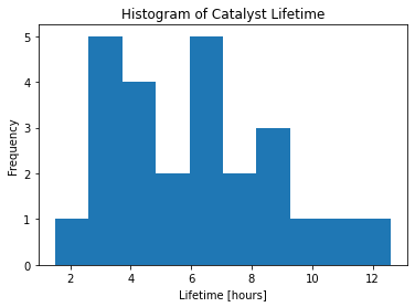
Note

Class Discussion: Are there outliers in the catalyst lifetime dataset?

another_example = [1.2, 2.3, 1.5, 1.4, 1.3, 1.6, 1.4, 1.7, 1.6, 1.5, 1.6]
plt.hist(another_example,color="red")
plt.title("Another Example")
plt.xlabel("Measured Variable")
plt.ylabel("Frequency")
plt.show()

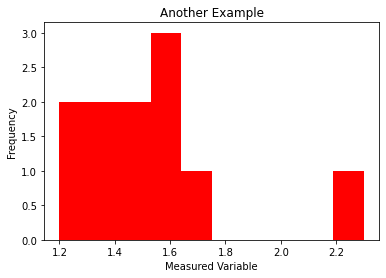
Note

Class Discussion: What about this dataset? Does it contain any outliers?

Another Example: Time Series Data.

Below are two plots of yield versus time data for two chemical processes.

#process 1
r = 0.2
sigma = 0.1
a = .8
b = .5
t = list(range(75))
yield1 = np.ones(75)
for i in t:
    temp1 = (1-r)*a*math.sin(i*b) + np.random.normal(0,sigma) + r*yield1[i-1]
    yield1[i-1] = np.min([np.max([temp1,0]),1])
    
#process 2
r = 0.2
sigma = 0.1
yield2 = np.ones(75)
for i in t:   
    temp2 = (1-r)*0.5 + np.random.normal(0,sigma) + r*yield2[i-1]
    yield2[i-1] = np.min([np.max([temp2,0]),1])
    


fig, axes = plt.subplots(nrows=1, ncols=2, figsize=(15, 5))
axes[0].plot(t, yield1, 'b.-')
axes[0].set_title('Process 1')
axes[0].set_xlabel('Time')
axes[0].set_ylabel('Yield')
axes[1].plot(t, yield2, 'b.-')
axes[1].set_title('Process 2')
axes[1].set_xlabel('Time')
axes[1].set_ylabel('Yield')
fig.tight_layout()

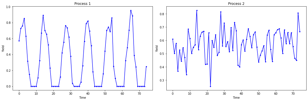
Note

Class Discussion: Can you use these data to calculate confidence intervals for the average yield of each process using a t-distribution?