Problem Set 3#

CBE 60258, University of Notre Dame. © Prof. Alexander Dowling, 2022

You may not distribution homework solutions without written permissions from Prof. Alexander Dowling.

Your Name and Email:

Import Libraries#

import math
import numpy as np
import scipy.stats as stats
from scipy import optimize

import sys
if "google.colab" in sys.modules:
    !wget "https://raw.githubusercontent.com/IDAES/idaes-pse/main/scripts/colab_helper.py"
    import colab_helper
    colab_helper.install_idaes()
    colab_helper.install_ipopt()

import pyomo.environ as pyo

1. Overflow and Algorithm Issues#

Over the past few years the lottery has reached amazing heights, in part due to the decrease in the individual odds of any set of numbers winning from 1/175M to 1/292.2M which begain in the fall of 2015. The all-time record payout drawing was on 1/13/16 and was worth $\$1.586B$ which, after taxes, was roughly $\$590M$. About $\$1B$ in tickets were sold at $\$2$ per ticket.

What is the probability there will be exactly $k$ winners for the lottery? If we assume that everyone choose to use the “computer option” to pick their numbers randomly, these probabilities can be computed from the binomial distribution.

Here is the probability mass function (PMF) of the binomial distribution:

(12)#\[\begin{equation} x(p,k,N) = \binom{N}{k} p^{k}(1-p)^{N-k} \end{equation}\]

It uses the binomial coefficient, which is another name for combinations:

(13)#\[\begin{equation} \binom{N}{k} = \frac{N!}{k!(N-k)!} \label{eq:2} \end{equation}\]

$N$ is the number of events (e.g., coin flips), $k$ is the number of “successes” (e.g., heads) and $p$ is the probability of success for a single event (e.g., heads for a single coin flip).

In this problem, you are given a function to calculate n choose r, shown below.

# define a function to calculate n choose r
def nCr(n,r):
    ''' Calculates n choose r
    Args:
        n : total number of items to choose from
        r : number of items to choose
    
    Return:
        Total number of combinations, calculated with factorial formula
    
    '''
    f = math.factorial
    # Note: Using integer division, //, prevents overflow errors in Python 3
#     return f(n) // f(r) // f(n-r)
    return f(n) / f(r) / f(n-r)
# End: define a function to calculate n choose r

Setup#

# Given data
# Number of people that purchased tickets
N = 500e6;
# Odds of winning
p = 1/(292.2e6);
# Net payout
net_pay = 590e6 # $

1a. Naive Calculation#

Let’s start with something simple: calculate the probability of exactly 2 winners.

We will first start with computing the binomial coefficient.

(14)#\[\begin{equation} \binom{N}{k} = \frac{N!}{k!(N-k)!} \end{equation}\]

Let’s divide this calculation into three pieces.

k = 2 # exactly 2 winners
print("k! = ",math.factorial(k))

Good, that worked. For the two remaining factorial calculations, we are going to add some extra code that will time out our calculation after 10 seconds.

# Configure the timer. You do not need to worry about anything in this box.
import signal
MAX_TIME = 1 # seconds. You may change this to 1 so that restart-run alls go faster

def signal_handler(signum, frame):
    raise Exception("Timed out! This cell took longer than "+str(MAX_TIME)+ " seconds.")

signal.signal(signal.SIGALRM, signal_handler)

signal.alarm(MAX_TIME)
print("N! = ",math.factorial(N))
signal.alarm(0)

Suggest at least one reason why math.factorial did not work for $N$ and $N-k$. Submit this discussion via Gradescope.

Do not fear, we can use Stirling’s approximation (https://en.wikipedia.org/wiki/Stirling’s_approximation).

\[ n! \approx \sqrt{2 \pi n} \left( \frac{n}{e} \right)^n \]

Finish the function below.

def stirling(n):
    ''' Approximate n!
    
    Args:
        n
        
    Returns:
        n_factorial    
    '''
    
    # Add your solution here

Now test your code by computing $10!$. Store your answer in the dictionary unit_test below.

unit_test = {}
unit_test['math.factorial'] = 0
unit_test['stirling'] = 0

# Add your solution here

# Removed autograder test. You may delete this cell.

We can now calculate try to calculate the probability of exactly 2 winners. We will break the calculation into several steps. Store your answer and the intermediates in the dictionary naive_calc.

## Naive calculation

k = 2

# Give our function stirling a nickname
f = stirling

naive_calc = {}
# k winners. Student update
naive_calc['p**k'] = 0

# (1-k) losers. Student update
naive_calc['(1-p)**(N-k)'] = 0

print(naive_calc)

# Binomial coefficient. Student update
naive_calc['nCk'] = 0

# Add your solution here

Alright, now let’s compute $\binom{N}{k}$

# N!. Student update
naive_calc['k!'] = 0

# Give our function stirling a nickname
f = stirling

# N!. Student update
naive_calc['N!'] = 0

# (N-k)!. Student update
naive_calc['(N-k)!'] = 0

# Add your solution here

print(naive_calc)

In a sentence, describe what happens (for example: did you see any warning messages?).

Discussion:

This problem prompts a brief discussion about floating point numbers. Computers use binary (0 or 1) to store all numbers. A bit is a single binary number.

A double-precision floating-point using 64 bits to store a decimal in scientific notation on a computer.

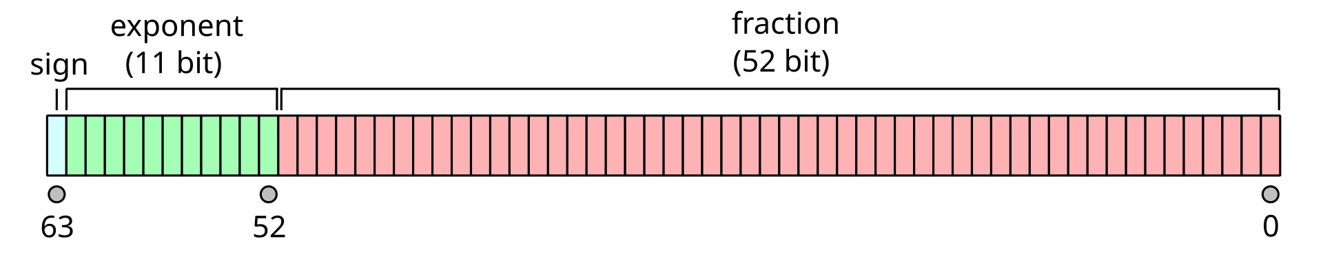
1 bit is used for the sign, 11 bits are used for exponent, and 52 bits are used for the fraction. Let’s focus on the exponent for a minute.

\[2^{11} = 2048\]

For many computers, this means that double-precision floating-point numbers must be between $10^{-1022}$ and $10^{1023}$. Here is the main take away: a computer cannot store arbitrarily large or small decimals with standard floating-point numbers. Python returns an overflow error if we exceed these bounds.

Determine the maximum number of lottery tickets ($N$) before Stirling’s approximation gives an overflow error. Store your answer as an integer in N_max. Hint: Start at 165 and start incrementing.

# Add your solution here
print(N_max)

# Add your solution here

1b. First Approximation#

Alright, we need to new strategy to approximate the binomial coefficient. We will now build an asymptotic approximations. You’ll see this idea again in Transport.

A mathematician would write:

(15)#\[\begin{equation} N >> k \implies N - k \approx N \end{equation}\]

Let’s take a minute to unpack this notation:

(16)#\[\begin{equation} \underbrace{N}_{\mathrm{lottery \ participants}} \qquad \underbrace{>>}_{\mathrm{much \ greater \ than}} \qquad \underbrace{k}_{\mathrm{lottery \ winners}} \qquad \underbrace{\implies}_{\mathrm{implies}} \qquad N - k \underbrace{\approx}_{\mathrm{approximately \ equals}} N \end{equation}\]

This allows us to make the following simplifications:

(17)#\[\begin{align} (N-k)! &= (N-k) \times (N-k-1) \times ... \times 1 \\ & = (N-k) \times (N-k-1) \times ... \times 1 \times \left(\frac{N \times (N-1) \times ... \times (N-k+1)}{N \times (N-1) \times ... \times (N-k+1)} \right)\\ & = \frac{N \times (N-1) \times ... \times (N-k+1) \times (N-k) \times (N-k-1) \times ... \times 1 } {N \times (N-1) \times ... \times (N -k + 1)} \end{align}\]

Notice that the numerator above is the definition of $N!$. We can use $N-k \approx N$ to simplify the demoniation to $N$ multiplied by itself $k$ times. Thus we have:

(18)#\[\begin{align} (N-k)! \approx \frac{N!}{N^{k}} \end{align}\]

Instructions: Starting with the definition for the binomial coefficient, show that:

(19)#\[\begin{equation} \label{finapp1} \binom{N}{k} \approx \frac{N^k}{k!} \end{equation}\]

In other words, write out all of the mathematical steps to go from $\binom{N}{k}$ to $\frac{N^k}{k!}$, similar to a proof. Submit your written work via Gradescope.

1c. Second Approximation#

Evaluation of $(1-p)^{N-k}$ can also be problematic. Construct a mathematical argument (i.e., proof) to establish that:

(20)#\[\begin{equation} (1-p)^{N-k} \approx e^{-Np} \end{equation}\]

Hint: Consider the following Taylor series expansion:

(21)#\[\begin{equation} \log_e (1 - p) = -p - \frac{p^2}{2} - \frac{p^3}{3} - ... \end{equation}\]

and truncate as follows:

(22)#\[\begin{equation} \label{tsep} \log_e (1 - p) \approx -p \end{equation}\]

The higher order terms ($p^2$, $p^3$, …) are incredibly small and can be ignored with negligible consequence.

Submit your written work via Gradescope.

1d. Take Two: Calculating the Odds#

Use the approximations from 1b and 1c to estimate the probability of exactly 0, 1, 2, 3, and 4 winners of the jackpoint.

Solve for the simplified, approximate governing formula on pencil and paper and submit via Gradescope.

Implement your equation in Python and save your answers as a list or numpy array named ref_prob.

## Refined calculation
# Add your solution here

for i in range(5):
    print("Probability of {0} winners: {1:0.4f}".format(i,ref_prob_fun(i)));

# Removed autograder test. You may delete this cell.

1e. Expected Return#

What is your expected return (after taxes) from purchasing just one of the 500 million tickets? Assume you elect for the lump sum payment. If more than one ticket “hits”, the jackpot is split evenly among the holders of the winning tickets.

Hint: You can calculate the expectation using $k=0$ through $k=4$ without introducing significant errors.

Solve for the governing formula on pencil and paper and submit via Gradescope.

Implement your equation in Python and save your answers as exp_pay.

## Expected return

# Add your solution here

# Display results
print('The expected return is $ {0:0.2f}'.format(exp_pay));

# Removed autograder test. You may delete this cell.

1f. Qualitative Analysis#

Interestingly, research has shown that if people pick their own numbers rather than letting the computer do it, the choices are highly non-random. In particular, people usually pick numbers from 0-31 (corresponding to birthdays) while the lottery numbers go from 0-69. In view of this, qualitatively answer the following questions:

Does the probability of any individual’s lottery ticket winning change?
Does the probability of getting multiple winners change (e.g., do you expect the payout to a winning ticket decrease due to splitting the prize)?
Does the probability of no one winning the lottery change?
For financial reasons, why are you better off letting the computer pick the numbers than picking birthdays?
Can you think of an even better strategy which would lead to higher winnings?

Write 1-3 sentences for each question. Submit your answer via Gradescope.

Discussion:

Fill in here.
Fill in here.
Fill in here.
Fill in here.
Fill in here.

2. Good and Bad Days at the Factory#

A bioreactor and separator produce 1000 batches of therapeutic proteins each day. Each batch has a 90% chance of meeting specifications. Using this information, answer the following:

2a. Probability Model#

Which probability distribution can you use to model the manufacturing process? What assumptions do you need to make?

Answer:

2b. Good Day#

If more than 890 batches in a day meet specifications, we will call it a good day.

Compute the probability of a good day and store it as the variable good. Hint: First you will need to write a function which calculates the total number of combinations of good and bad batches in a day.

# Define function
# Add your solution here

# probability of more than 890 batches meet specifications
# Add your solution here

# Removed autograder test. You may delete this cell.

2c. Bad Day#

Likewise, we will call a day with 890 or fewer on specification batches a bad day.

Compute the probability of a bad day and store your answer in the variable bad. Hint: How can you do this quickly using your previous answer?

# Add your solution here

# Removed autograder test. You may delete this cell.

2d. Bad Days in a Work Week#

Using your answer from above, compute the probability of 0, 1, 2, …, 5 bad days in a 5-day work week. Store your answer as a list called weekly.

# Add your solution here

# Removed autograder test. You may delete this cell.

# Extract indices
x = sorted(m.x)
t = sorted(m.t)

# Create numpy arrays to hold the solution
xgrid = np.zeros((len(t), len(x)))
# Hint: define tgrid and Tgrid the same way
# Add your solution here

# Loop over time
for i in range(0, len(t)):
    # Loop over space
    for j in range(0, len(x)):
        # Copy values
        xgrid[i,j] = x[j]
        tgrid[i,j] = t[i]
        # Hint: how to access values from Pyomo variable m.T?
        # Add your solution here

# Create a 3D wireframe plot of the solution
# Hint: consult the matplotlib documentation
# https://matplotlib.org/stable/gallery/mplot3d/wire3d.html

# Add your solution here

3. Portfolio Data Analysis#

Portfolio management is a classic example of quadratic programming (optimization). The idea is to find the optimal blend of investments that achieves a specified rate of return (or better) while minimizing the variance in rate of return. In this problem, you will use your skills in statistical analysis to analyze the stock data.

Historical Stock Data#

Historical daily adjusted closing prices for the last five years (obtained from Yahoo! Finance) are available for the $N=5$ stocks listed in table below. (We are actually considering index funds, but this detail does not change the analysis.)

Symbol	Name
GSPC	S&P 500
DJI	Dow Jones Industrial Average
IXIC	NASDAQ Composite
RUT	Russell 2000
VIX	CBOE Volatility Index

3a. Return Rate#

You are given a Stock_Data.csv file. Using the stock data, calculate the 1-day return rate:

(23)#\[\begin{equation} r_{t,i} = \frac{p_{t+1,i} - p_{t,i}}{p_{t,i}} \end{equation}\]

where $p_{t+1,i}$ and $p_{t,i}$ are the Adjusted Closing Prices at the end of days $t+1$ and $t$, respectively, for stock $i$. These results are stored in matrix R. Hint: Use Pandas.

# This is the long path to the folder containg data files on GitHub (for the class website)
data_folder = 'https://raw.githubusercontent.com/ndcbe/data-and-computing/main/noteboohttps://raw.githubusercontent.com/ndcbe/data-and-computing/main/notebooks/data/'

# Load the data file into Pandas
df_adj_close = pd.read_csv(data_folder + 'Stock_Data.csv')

# Add your solution here

3b. Visualization#

Plot the single day return rates for the 5 stocks you obtain in the previous section and check if you obtain the following profiles:

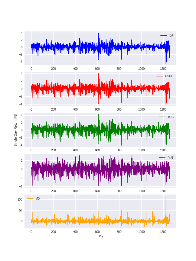
The first plot is made for you.

# Create figure
plt.figure(figsize=(9,15))

# Create subplot for DJI
plt.subplot(5,1,1)
plt.plot(R["DJI"]*100,color="blue",label="DJI")
plt.legend(loc='best')

# Add your solution here

# Show plot
plt.show()

3c. Covariance and Correlation Matrices#

Write Python code to:

Calculate $\bar{r}$, the average 1-day return for each stock. Store this as the variable R_avg.
Calculate $\Sigma_{r}$, the covariance matrix of the 1-day returns. This matrix tells us how returns for each stock vary with each other (which is important because they are correlated!). Hint: pandas has a function cov
Calculate the correlation matrix for the 1-day returns. Hint: pandas has a function corr.

Looking at the correlation matrix, answer the follwing questions:

Which pair of stocks have the highest positive correlation?
Which pair of stocks have the highest negative correlation?
Which pair of stocks have the lowest absolute correlation?

Hint: Read ahead in the class website for more information on correlation and covariance

Please write one or two sentences for each of the above questions:

Fill in here
Fill in here
Fill in here

# Add your solution here

# Removed autograder test. You may delete this cell.

3d. Markowitz Mean/Variance Portfolio Model#

The Markowitz mean/variance model, shown below, computes the optimal allocation of funds in a portfolio:

(24)#\[\begin{align} \min_{{x} \geq {0}} \qquad & z:= {x}^T \cdot {\Sigma_r} \cdot {x} \\ \text{s.t.} \qquad & {\bar{r}}^T \cdot {x} \geq \rho \\ & \sum_{i =1}^N x_i = 1 \end{align}\]

where $x_i$ is the fraction of funds invested in stock $i$ and $x = [x_1, x_2, ..., x_N]^T$. The objective is to minimize the variance of the return rate. (As practice for the next exam, try deriving this from the error propagation formulas.) This requires the expected return rate to be at least $\rho$. Finally, the allocation of funds must sum to 100%.

Write Python code to solve for $\rho = 0.08\%.$ Report both the optimal allocation of funds and the standard deviation of the return rate. Hint:

Be mindful of units.
You can solve with problem using the Pyomo function given below
$:=$ means ‘’defined as’’

Store your answer in std_dev.

R_avg_tolist = R_avg.values.tolist()
Cov_list = Cov.values.tolist()

# Optimization Problem
def create_model(rho,R_avg,Cov):
    
    '''
    This function solves for the optimal allocation of funds in a portfolio 
    by minimizing the variance of the return rate
    
    Arguments:
        rho: required portfolio expected return
        Ravg: average return rates (list)
        Cov: covariance matrix
        
    Returns:
        m: Pyomo concrete model
    
    '''
    
    m = pyo.ConcreteModel()
    init_x = {}
    m.idx = pyo.Set(initialize=[0,1,2,3,4])
    for i in m.idx:
        init_x[i] = 0
    m.x = pyo.Var(m.idx,initialize=init_x,bounds=(0,None))
    
    def Obj_func(m):
        b = []
        mult_result = 0
        for i in m.idx:
            a = 0
            for j in m.idx:
                a+= m.x[j]*Cov[j][i]
            b.append(a)
        for i in m.idx:
            mult_result += b[i]*m.x[i]
        
        return mult_result
    m.OBJ = pyo.Objective(rule=Obj_func)
    
    def constraint1(m):
        # Add your solution here

    m.C1 = pyo.Constraint(rule=constraint1)
    
    def constraint2(m):
        # Add your solution here

    m.C2 = pyo.Constraint(rule=constraint2)
    
    return m

rho = 0.0008
model1 = create_model(rho,R_avg_tolist,Cov_list)

#Solve Pyomo in the method learned in Class 11

# Add your solution here

# Removed autograder test. You may delete this cell.

3e. Volatility and Expected Return Tradeoff#

We will now perform sensitivity analysis of the optimization problem in 3d to characterize the tradeoff between return and risk.