14.1. Correlation, Covariance, and Independence#
Further Reading: §7.1 Navidi (2015)
14.1.1. Learning Objectives#
After studying this notebook and your lecture notes, you should be able to:
Interpret correlation coefficients.
Understand the relationship between correlation, covariance, and independence.
Determine if two variables are linearly associated.
import numpy as np
import matplotlib.pyplot as plt
14.1.2. Correlation#
Correlation Coefficient:
The numerator is also known as \(cov(X,Y)\).
Sample Correlation:
Correlation coefficient is dimensionless.
It remains unchanged when:
Scaling a variable by a positive constant.
Adding a constant to a varible.
Interchanging the values of x and y.
Important Notes:
Correlation coefficient only measures linear association.
Correlation coefficient can be misleading when outliers are present.
Correlation is NOT causation.
Controlled experiments reduce the risk of confounding.
Home Activity
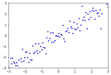
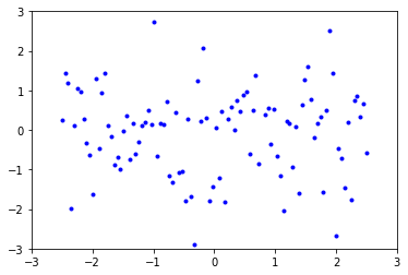
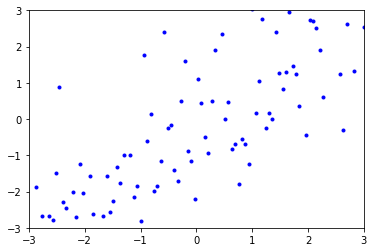
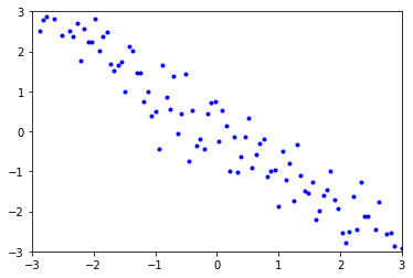
In the following cell, add A-E to the proper strings to correctly match each graph with its correlation coefficient.
# Correlation coefficient of -0.95
ans1 = ''
# Correlation coefficient of -0.50
ans2 = ''
# Correlation coefficient of 0.00
ans3 = ''
# Correlation coefficient of 0.50
ans4 = ''
# Correlation coefficient of 0.95
ans5 = ''

# Add your solution here
Graph A:
Graph B:
Graph C:

Graph D:
Graph E:
14.1.3. Covariance#
Often data are not independent because of observation error (or because the variables are related).
Covariance measures the linear relationship between two random variables.
14.1.4. Independence#
If \(cov(X,Y) = 0 = \rho_{X,Y}\), then \(X\) and \(Y\) are uncorrelated.
If \(X\) and \(Y\) are independent, then \(X\) and \(Y\) are uncorrelated.
It is possible for \(X\) and \(Y\) to be uncorrelated and NOT independent.