6.1. Modeling Systems of Nonlinear Equations: Flash Calculation Example#
6.1.1. Learning Objectives#
After studying this notebook, completing the activities, and asking questions in class, you should be able to:
Use Newton’s Method to model and solve systems of nonlinear equations in python.
Understand and interpret the results of Newton’s Method.
import numpy as np
6.1.2. Flash Calculations are Central to Chemical Engineering#
Many chemical engineering problems require solving nonlinear systems of equations. For example, we will consider the general two-phase flash calculation without the dilute assumption. The flash calculation is the main building block for steady-state process analysis. It is arguably one of the most important calculations in chemical engineering.
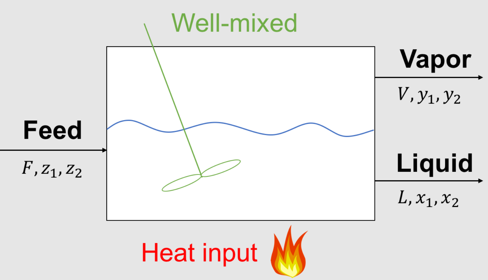 Figure 1: Generic well-mixed two-phase flash system. This simple example will resurface throughout your ChE education to illustrate new concepts.
Parameters (given):
\(F\) feed inlet flowrate, mol/time or kg/time
\(z_1\) composition of species 1 in feed, mol% or mass%
\(z_2\) composition of species 2 in feed, mol% or mass%
\(K_1\) partition coefficient for species 1, mol%/mol% or mass% / mass%
\(K_2\) partition coefficient for species 2, mol%/mol% or mass% / mass%
Variables (unknown):
\(L\) liquid outlet flowrate, mol/time or kg/time
\(x_1\) composition of species 1 in liquid, mol% or mass%
\(x_2\) composition of species 2 in liquid, mol% or mass%
\(V\) vapor outlet flowrate, mol/time or kg/time
\(y_1\) composition of species 1 in vapor, mol% or mass%
\(y_2\) composition of species 2 in vapor, mol% or mass%
6.1.3. Partition Coefficients#
We can model the vapor-liquid equilibrium using partition coefficients \(K_1\) and \(K_2\):
and
or more compactly
where \(\forall\) means for all. This one line says to duplicate the equation for \(i=1\) and \(i=2\).
Looking Ahead: In thermodynamics, you will learn about complex models to predict how \(K\) changes with temperature, pressure, and composition. For now, we will just assume the partition coefficient is constant or give you a formula to calculate it.
Simplification: Assume the system is maintained at a desired outlet temperature \(T\) and we know equilibrium coefficients \(K_1\) and \(K_2\) at this temperature. For now, we do not want to calculate the amount of heat need to obtain \(T\).
Home Activity
Write down one question about this problem description you can ask a friend, the TAs, or instructor during class.
6.1.4. Full Mathematical Model#
We will say a nonlinear model is in canonical form when we can express it as \(c(\mathbf{z}) = \mathbf{0}\). Here \(c(\cdot)\) is a vector-valued function. We say the model is square if the number of variables is the same as the number of equations (dimensions of \(c\)).
Class Activity
With a partner, propose a mathematical model to calculate the unknown flow rates and compositions. Hint: how many equations do we need?
6.1.5. Solve Nonlinear System with Python#
Now that we have the mathematical model, we need to write a Python function to calculate the residuals.
Class Activity
Complete the residual calculations in the function below.
# First, we need to define a function that returns the residual for our system of equations
def my_c2(x):
    ''' Nonlinear system of equations in canonical form c(x) = 0

    Arg:
        x: vector of variables

    Returns:
        r: residual, c(x)

    '''

    # Initialize residuals
    r = np.zeros(6)

    # given data
    F = 1.0
    z1 = 0.5
    z2 = 0.5
    K1 = 3
    K2 = 0.05

    # copy values from x to more meaningful names
    L = x[0]
    V = x[1]
    x1 = x[2]
    x2 = x[3]
    y1 = x[4]
    y2 = x[5]

    # equation 1: overall mass balance
    r[0] = V + L - F

    # equations 2 and 3: component mass balances
    # Add your solution here

    # equation 4 and 5: equilibrium
    # Add your solution here

    # equation 6: summation
    r[5] = (y1 + y2) - (x1 + x2)
    # This is known as the Rachford-Rice formulation for the summation constraint

    return r
Now let’s define an initial guess for the variables. We’ll test our function by evaluating it at the initial guess.
# Next we define an initial guess
# We'll guess an equal split between liquid and vapor phases
# Based on the values of K (and experience), we see that the vapor phase will become enriched in the first component
# We will come back to why a good initial guess is so important
x0 = np.array([0.5, 0.5, 0.55, 0.45, 0.65, 0.35])

my_c2(x0)
array([ 0. , 0.1 , -0.1 , -1. , 0.3275, 0. ])
In the next notebook, we will study the details of Newton’s method for solving systems of nonlinear equations. Below is the code we’ll study then. We’ll just use it now.
# You do not need to understand how this code works right now.
# We will discuss Newton's Method more in depth in the next notebook.
def Jacobian(f,x,delta = 1.0e-7):
    '''Approximate Jacobian using forward finite difference

    Args:
        f: vector-valued function
        x: point to build approximation J(x) around
        delta: finite difference step size

    Returns:
        J: square Jacobian matrix (approximation)

    '''
    # Determine size
    N = x.size

    #Evaluate function f at x
    fx = f(x) #only need to evaluate this once

    # Make sure f is square (no. inputs = no. outputs)
    try:
        assert N == fx.size, "Your problem is not square!"
    except AssertionError:
        print("x = ",x)
        print("fx = ",fx)


    # Allocate empty matrix
    J = np.zeros((N,N))

    idelta = 1.0/delta #division is slower than multiplication
    x_perturbed = x.copy() #copy x to add delta

    # Loop over elements of x and columns of J
    for i in range(N):
        # Perturb (apply step) to element i of x
        x_perturbed[i] += delta

        # Approximate column in Jacobian
        col = (f(x_perturbed) - fx) * idelta

        # Reset element of x
        x_perturbed[i] = x[i]

        # Save results
        J[:,i] = col
    # end for loop
    return J

def newton_system(f,x0,exact_Jac=None,delta=1E-7,epsilon=1.0e-6, LOUD=False):
    """Find the root of the function f via exact or inexact Newton-Raphson method
    Args:
        f: function to find root of
        x0: initial guess
        exact_Jac: function to calculate J. If None, use finite difference
        delta: finite difference tolerance. Only used if J is not specified
        epsilon: tolerance

    Returns:
        estimate of root
    """

    x = x0
    if (LOUD):
        print("x0 =",x0)
    iterations = 0
    fx = f(x)
    while (np.linalg.norm(fx) > epsilon):
        if exact_Jac is None:
            # Use finite difference
            J = Jacobian(f,x,delta)
        else:
            J = exact_Jac(x)

        RHS = -fx;

        # solve linear system
        # We could have used GaussElimPivotSolve here instead
        delta_x = np.linalg.solve(J,RHS)

        # Check if GE returned any NaN values
        if np.isnan(delta_x).any():
            print("Gaussian Elimination Failed!")
            print("J = \n",J,"\n")
            print("J is rank",np.linalg.matrix_rank(J),"\n")
            print("RHS = ",RHS)
        x = x + delta_x
        fx = f(x)
        if (LOUD):
            print("\nIteration",iterations+1,": x =",x,"\n norm(f(x)) =",np.linalg.norm(fx))
        iterations += 1
    print("\nIt took",iterations,"iterations")
    return x #return estimate of root
We can now solve the nonlinear system of equations.
# We can now solve with Newton's method
x = newton_system(my_c2, x0,LOUD=True)

# Check that residual is zero at the solution
print("\nChecking residuals")
print("c(x) = \n",my_c2(x),"\n")

# And finally report the answer
print("L = ",x[0])
print("V = ",x[1])
print("x1 = ",x[2])
print("x2 = ",x[3])
print("y1 = ",x[4])
print("y2 = ",x[5])
x0 = [0.5  0.5  0.55 0.45 0.65 0.35]

Iteration 1 : x = [ 1.94067797 -0.94067797  0.3220339   0.6779661   0.9661017   0.03389831]
 norm(f(x)) = 1.1084980482929316

Iteration 2 : x = [0.72368421 0.27631579 0.3220339  0.6779661  0.96610169 0.03389831]
 norm(f(x)) = 3.0340609559661354e-09

It took 2 iterations

Checking residuals
c(x) =
 [ 2.70226908e-09 -2.81673573e-11  1.37930212e-09  1.11022302e-16
 -6.93889390e-18  0.00000000e+00]

L =  0.723684213574546
V =  0.27631578912772303
x1 =  0.32203389786997366
x2 =  0.677966100778892
y1 =  0.966101693609921
y2 =  0.033898305038944594
A few highlights from the output:
Newton’s method only needs two iterations to converge! We’ll see more in the Newton’s Method in One Dimension notebook about why Newton’s method is so efficient on this problem (most of the time).
The residuals are all near zero (less than \(10^{-8}\)) at the solution. This means all of the model equations are satisfied.
The flowrates and compositions make sense (not negative, etc.)