10.4. Jointly Continuous Random Variables

10.4.1. Learning Objectives

After attending class, completing these activities, asking questions, and studying notes, you should be able to:

• Understand the difference between jointly distributed and jointly continuous random variables.

• Explain what joint and marginal probability density functions are and how to calculate them.

import matplotlib.pyplot as plt
import matplotlib.patches as mpatches

Note

Unlinke jointly distributed random variables that can only take on certain values, jointly continuous random variables can take on any value within a specified range. This changes the functions from mass to density functions as we are looking at a range of values rather than specific values.

10.4.2. Key Equations

Joint Probability Density Function:

\[f(x,y) = P(X=x \textrm{ and } Y=y)\]

\[P(a \leq X \leq b \textrm{ and } c \leq Y \leq d) = \int_a^b \int_c^d f(x,y) dy dx\]

Note that…

\[\int_{-\infty}^{\infty} \int_{-\infty}^{\infty} f(x,y) = 1\]

Both joint probability density and mass functions generalize to higher dimensions.

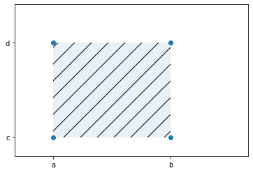
Below is a visual representation with \(f(x,y)\) being the shaded region.

fig, ax = plt.subplots()
plt.scatter([1,1,4,4],[1,6,1,6])
plt.xlim(0,6)
plt.ylim(0,8)
plt.xticks([1,4])
plt.yticks([1,6])
ax.set_xticks([1,4],labels=['a','b'])
ax.set_yticks([1,6],labels=['c','d'])
rect=mpatches.Rectangle((1,1),3,5, fill=True,alpha=0.1,hatch='/')
plt.gca().add_patch(rect)
plt.show()

Marginal Probability Density Function:

\[f_X(x) = \int_{-\infty}^{\infty} f(x,y) dy\]

\[f_Y(y) = \int_{-\infty}^{\infty} f(x,y) dx\]

While joint probability is with respect to two events occurring simultaneously, marginal probability is the probability of an event occurring regardless of the outcome of another variable.