6.5. Newton-Raphson Methods for Systems of Equations#
6.5.1. Learning Objectives#
After studying this notebook, completing the activities, and asking questions in class, you should be able to:
Extend Newton’s Method to multiple dimensions through the flash example.
Know how to assemble a Jacobian matrix and what that means.
Understand how to use a finite difference formula to approximate the Jacobian matrix.
Apply Multivariate Newton’s Method to the flash problem.
import numpy as np
6.5.2. Motivation: Flash Problem Revisited#
Recall the flash problem from the Modeling Systems of Nonlinear Equations notebook:
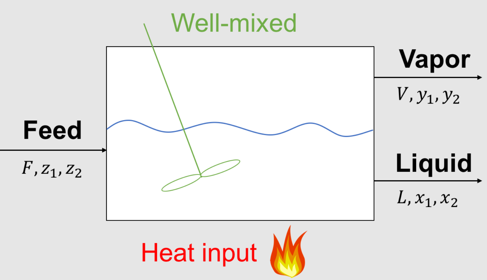
Parameters (given):
\(F\) feed inlet flowrate, mol/time or kg/time
\(z_1\) composition of species 1 in feed, mol% or mass%
\(z_2\) composition of species 2 in feed, mol% or mass%
\(K_1\) partion coefficient for species 1, mol%/mol% or mass% / mass%
\(K_2\) partion coefficient for species 2, mol%/mol% or mass% / mass%
Variables (unknown):
\(L\) liquid outlet flowrate, mol/time or kg/time
\(x_1\) composition of species 1 in liquid, mol% or mass%
\(x_2\) composition of species 2 in liquid, mol% or mass%
\(V\) vapor outlet flowrate, mol/time or kg/time
\(y_1\) composition of species 1 in vapor, mol% or mass%
\(y_2\) composition of species 2 in vapor, mol% or mass%
How to solve the flash problem and other multidimensional problem with \(n\) unknown variables and \(n\) nonlinear equations?
6.5.3. Extending Newton’s Method to Multiple Dimensions#
Say that we have a function of \(n\) variables \(\mathbf{x} = (x_1, \dots x_n):\)
the root is \(\mathbf{F}(\mathbf{x}) = \mathbf{0}.\) For this scenario we know longer have a tangent line at point \(\mathbf{x}\), rather we have an \(n\)-dimensional tangent vector that is defined using the Jacobian matrix
to define the tangent vector as \(\mathbf{J}(\mathbf{x})\mathbf{x}\). Now we reformulate Newton’s method for a single equation
as
The multidimensional analog of this is
Note this is a linear system of equations to solve to get a vector of changes for each \(x\): \(\delta = x_{i+1} - x_{i}.\) Therefore, in each step we solve the system
and set
In multidimensional root finding we can observe the importance of having a small number of iterations: we need to solve a linear system of equations at each iteration. If this system is large, the time to find the root could be prohibitively long.
To demonstrate how Newton’s method works for a multi-dimensional function.
6.5.4. Two Phase, Single Feed Phase Problem#
6.5.5. Mathematical Model#
Feed Specifications: \(F = 1.0\) mol/s, \(z_1\) = 0.5 mol/mol, \(z_2\) = 0.5 mol/mol
Given Equilibrium Data: \(K_1\) = 3 mol/mol, \(K_2\) = 0.05 mol/mol
Overall Material Balance
Component Mass Balances
Thermodynamic Equilibrium
Summation
6.5.6. Convert to Canonical Form#
How to convert these equations to \(\mathbf{F}(\mathbf{x}) = 0\)?
with \(\mathbf{x} = (L, V, x_1, x_2, y_1, y_2).\)
Some people use \(\mathbf{F}(\mathbf{x}) = 0\) and others use \(c(x) = 0\) for canonical form. They mean the same thing.
Home Activity
Verify each equation in the model above was correctly transcribed into the function below.
def my_f(x):
    ''' Nonlinear system of equations in conancial form F(x) = 0
    Copied from previous notebook.

    Arg:
        x: vector of variables

    Returns:
        r: residual, F(x)

    '''

    # Initialize residuals
    r = np.zeros(6)

    # given data
    F = 1.0
    z1 = 0.5
    z2 = 0.5
    K1 = 3
    K2 = 0.05

    # copy values from x to more meaningful names
    L = x[0]
    V = x[1]
    x1 = x[2]
    x2 = x[3]
    y1 = x[4]
    y2 = x[5]

    # equation 1: overall mass balance
    r[0] = V + L - F

    # equations 2 and 3: component mass balances
    r[1] = V*y1 + L*x1 - F*z1
    r[2] = V*y2 + L*x2 - F*z2

    # equation 4 and 5: equilibrium
    r[3] = y1 - K1*x1
    r[4] = y2 - K2*x2

    # equation 6: summation
    r[5] = (y1 + y2) - (x1 + x2)
    # This is known as the Rachford-Rice formulation for the summation constraint

    return r
6.5.7. Assemble Jacobian Matrix (Analytic)#
The Jacobian is
which evaluates to
We can tediously program a function to evaluate the Jacobian.
Home Activity
Verify the second row in the Jacobian was calculated properly.
def my_J(x):
    '''Jacobian matrix for two phase flash problem

    Arg:
        x: vector of variables

    Returns:
        J: square Jacobian matrix
    '''

    # allocate matrix of zeros
    J = np.zeros((6,6))

    # given data
    F = 1.0
    z1 = 0.5
    z2 = 0.5
    K1 = 3
    K2 = 0.05

    # copy values from x to more meaningful names
    L = x[0]
    V = x[1]
    x1 = x[2]
    x2 = x[3]
    y1 = x[4]
    y2 = x[5]

    # first row (overall material balance)
    J[0,0] = 1
    J[0,1] = 1

    # second row (component 1 material balance)
    J[1,0] = x1
    J[1,1] = y1
    J[1,2] = L
    J[1,4] = V

    # third row (component 2 material balance)
    J[2,0] = x2
    J[2,1] = y2
    J[2,3] = L
    J[2,5] = V

    # fourth row (equilibrium for component 1)
    J[3,2] = -K1
    J[3,4] = 1

    # fifth row (equilibrium for component 2)
    J[4,3] = -K2
    J[4,5] = 1

    # sixth row (summation equation)
    J[5,2] = -1
    J[5,3] = -1
    J[5,4] = 1
    J[5,5] = 1

    return J
Unit Test: Immediately after we create a function, we should test it. Let’s reuse the same initial guess as in this previous notebook.
\(L = 0.5\), \(V = 0.5\), \(x_1 = 0.55\), \(x_2 = 0.45\), \(y_1 = 0.65\), \(y_2 = 0.35\)
Jacobian structure copied from above:
x0 = np.array([0.5, 0.5, 0.55, 0.45, 0.65, 0.35])
print("J(x0) = \n",my_J(x0))
J(x0) =
 [[ 1.    1.    0.    0.    0.    0.  ]
 [ 0.55  0.65  0.5   0.    0.5   0.  ]
 [ 0.45  0.35  0.    0.5   0.    0.5 ]
 [ 0.    0.   -3.    0.    1.    0.  ]
 [ 0.    0.    0.   -0.05  0.    1.  ]
 [ 0.    0.   -1.   -1.    1.    1.  ]]
6.5.8. First Iteration#
print("F(x0) = \n",my_f(x0),"\n")
print("J(x0) = \n",my_J(x0),"\n")
F(x0) =
 [ 0.      0.1    -0.1    -1.      0.3275  0.    ]

J(x0) =
 [[ 1.    1.    0.    0.    0.    0.  ]
 [ 0.55  0.65  0.5   0.    0.5   0.  ]
 [ 0.45  0.35  0.    0.5   0.    0.5 ]
 [ 0.    0.   -3.    0.    1.    0.  ]
 [ 0.    0.    0.   -0.05  0.    1.  ]
 [ 0.    0.   -1.   -1.    1.    1.  ]]
We now need to solve the linear system:
Let’s use Gaussian elimination. We’ll start by copying the code from the Gauss Elimination notebook:
Home Activity
Please read through the docstrings for each function below.
import numpy as np

def BackSub(aug_matrix,z_tol=1E-8):
    """back substitute a N by N system after Gauss elimination

    Args:
        aug_matrix: augmented matrix with zeros below the diagonal [numpy 2D array]
        z_tol: tolerance for checking for zeros below the diagonal [float]
    Returns:
        x: length N vector, solution to linear system [numpy 1D array]
    """
    [Nrow, Ncol] = aug_matrix.shape
    try:
        # check the dimensions
        assert Nrow + 1 == Ncol
    except AssertionError:
        print("Dimension checks failed.")
        print("Nrow = ",Nrow)
        print("Ncol = ",Ncol)
        raise

    assert type(z_tol) is float, "z_tol must be a float"

    # check augmented matrix is all zeros below the diagonal
    for r in range(Nrow):
        for c in range(0,r):
            assert np.abs(aug_matrix[r,c]) < z_tol, "\nWarning! Nonzero in position "+str(r)+","+str(c)

    # create vector of zeros to store solution
    x = np.zeros(Nrow)

    # loop over the rows starting at the bottom
    for row in range(Nrow-1,-1,-1):
        RHS = aug_matrix[row,Nrow] # far column

        # loop over the columns to the right of the diagonal
        for column in range(row+1,Nrow):

            # substract, i.e., substitute the already known values
            RHS -= x[column]*aug_matrix[row,column]

        # compute the element of x corresponding to the current row
        x[row] = RHS/aug_matrix[row,row]

    ### END SOLUTION
    return x

def swap_rows(A, a, b):
    """Rows two rows in a matrix, switch row a with row b

    args:
    A: matrix to perform row swaps on
    a: row index of matrix
    b: row index of matrix

    returns: nothing

    side effects:
    changes A to rows a and b swapped
    """

    # A negative index will give unexpected behavior
    assert (a>=0) and (b>=0)
    N = A.shape[0] #number of rows
    assert (a<N) and (b<N) #less than because 0-based indexing

    # create a temporary variable to store row a
    temp = A[a,:].copy()

    # move row b values into the location of row a
    A[a,:] = A[b,:].copy()

    # move row a values (stored in temp) into the location of row a
    A[b,:] = temp.copy()

def GaussElimPivotSolve(A,b,LOUD=False):
    """create a Gaussian elimination with pivoting matrix for a system

    Args:
        A: N by N array
        b: array of length N
    Returns:
        solution vector in the original order
    """

    # checks dimensions
    [Nrow, Ncol] = A.shape
    assert Nrow == Ncol
    N = Nrow


    #create augmented matrix
    aug_matrix = np.zeros((N,N+1))
    aug_matrix[0:N,0:N] = A
    aug_matrix[:,N] = b
    #augmented matrix is created

    #create scale factors
    s = np.zeros(N)
    count = 0
    for row in aug_matrix[:,0:N]: #don't include b
        s[count] = np.max(np.fabs(row))
        count += 1

    # print diagnostics if requested
    if LOUD:
        print("s =",s)
        print("Original Augmented Matrix is\n",aug_matrix)

    #perform elimination
    for column in range(0,N):

        ## swap rows if needed
        # find largest position
        largest_pos = (np.argmax(np.fabs(aug_matrix[column:N,column]/
                                         s[column:N])) + column)

        # check if current column is largest position
        if (largest_pos != column):
            # if not, swap rows
            if (LOUD):
                print("Swapping row",column,"with row",largest_pos)
                print("Pre swap\n",aug_matrix)
            swap_rows(aug_matrix,column,largest_pos)

            #re-order s
            tmp = s[column]
            s[column] = s[largest_pos]
            s[largest_pos] = tmp
            if (LOUD):
                print("A =\n",aug_matrix)
                print("new_s =\n", s)

        #finish off the row
        for row in range(column+1,N):
            mod_row = aug_matrix[row,:]
            mod_row = mod_row - mod_row[column]/aug_matrix[column,column]*aug_matrix[column,:]
            aug_matrix[row] = mod_row

    #now back solve
    if LOUD:
        print("Final aug_matrix is\n",aug_matrix)
    x = BackSub(aug_matrix)
    return x
And now let’s solve the linear system, copied again for clarity:
delta_1 = GaussElimPivotSolve(my_J(x0), -my_f(x0))
print("delta_1 =",delta_1)
delta_1 = [ 1.44067797 -1.44067797 -0.2279661 0.2279661 0.31610169 -0.31610169]
Finally, we need to calculate \(\mathbf{x_1}\):
x1 = x0 + delta_1
print("x1 = ",x1)
x1 = [ 1.94067797 -0.94067797 0.3220339 0.6779661 0.96610169 0.03389831]
The results for multivariate Newton’s method matches the single variable case. Division is replaced with solving a linear system of equations.
Home Activity
Notice anything strange about \(\mathbf{x}_1\)? Recall that \(\mathbf{x} = (L, V, x_1, x_2, y_1, y_2)\). Write a sentence below.
Write your sentence here:
6.5.9. Finite Difference to Approximate the Jacobian Matrix#
Assembling the Jacobian matrix for each problem is tedious and error prone. Instead, we can apply finite difference to each element of \(\mathbf{x}\) to built the Jacobian matrix column by column.
Class Activity
With a partner, use a picture of Jacobian matrix to explain the main steps of the code below.
def Jacobian(f,x,delta = 1.0e-7):
    '''Approximate Jacobian using forward finite difference

    Args:
        f: vector-valued function
        x: point to build approximation J(x) around
        delta: finite difference step size

    Returns:
        J: square Jacobian matrix (approximation)

    '''
    # Determine size
    N = x.size

    #Evaluate function f at x
    fx = f(x) #only need to evaluate this once

    # Make sure f is square (no. inputs = no. outputs)
    try:
        assert N == fx.size, "Your problem is not square!"
    except AssertionError:
        print("x = ",x)
        print("fx = ",fx)


    # Allocate empty matrix
    J = np.zeros((N,N))

    idelta = 1.0/delta #division is slower than multiplication
    x_perturbed = x.copy() #copy x to add delta

    # Loop over elements of x and columns of J
    for i in range(N):
        # Perturb (apply step) to element i of x
        x_perturbed[i] += delta

        # Approximate column in Jacobian
        col = (f(x_perturbed) - fx) * idelta

        # Reset element of x
        x_perturbed[i] = x[i]

        # Save results
        J[:,i] = col
    # end for loop
    return J
Unit Test: Immediately after we create a function, we need to test it. Let’s use or flash problem as a unit test.
print("*** Analytic ***")
print("J(x0) = \n",my_J(x0),"\n")

print("\n\n*** Finite Difference ***")
print("J(x0) = \n",Jacobian(my_f,x0),"\n")
*** Analytic ***
J(x0) =
 [[ 1.    1.    0.    0.    0.    0.  ]
 [ 0.55  0.65  0.5   0.    0.5   0.  ]
 [ 0.45  0.35  0.    0.5   0.    0.5 ]
 [ 0.    0.   -3.    0.    1.    0.  ]
 [ 0.    0.    0.   -0.05  0.    1.  ]
 [ 0.    0.   -1.   -1.    1.    1.  ]]


*** Finite Difference ***
J(x0) =
 [[ 1.    1.    0.    0.    0.    0.  ]
 [ 0.55  0.65  0.5   0.    0.5   0.  ]
 [ 0.45  0.35  0.    0.5   0.    0.5 ]
 [ 0.    0.   -3.    0.    1.    0.  ]
 [ 0.    0.    0.   -0.05  0.    1.  ]
 [ 0.    0.   -1.   -1.    1.    1.  ]]
6.5.10. Putting it all together: Multivariate Newton’s Method#
We can now stick together i) solving a linear system, and ii) finite difference into a multivariate Newton’s method solver.
def newton_system(f,x0,exact_Jac=None,delta=1E-7,epsilon=1.0e-6, LOUD=False):
    """Find the root of the function f via exact or inexact Newton-Raphson method
    Args:
        f: function to find root of
        x0: initial guess
        exact_Jac: function to calculate J. If None, use finite difference
        delta: finite difference tolerance. Only used if J is not specified
        epsilon: tolerance

    Returns:
        estimate of root
    """

    x = x0
    if (LOUD):
        print("x0 =",x0)
    iterations = 0
    fx = f(x)
    while (np.linalg.norm(fx) > epsilon):
        if exact_Jac is None:
            # Use finite difference
            J = Jacobian(f,x,delta)
        else:
            J = exact_Jac(x)

        RHS = -fx;

        # solve linear system
        # We could have used GaussElimPivotSolve here instead
        delta_x = np.linalg.solve(J,RHS)

        # Check if GE returned any NaN values
        if np.isnan(delta_x).any():
            print("Gaussian Elimination Failed!")
            print("J = \n",J,"\n")
            print("J is rank",np.linalg.matrix_rank(J),"\n")
            print("RHS = ",RHS)
        x = x + delta_x
        fx = f(x)
        if (LOUD):
            print("\nIteration",iterations+1,": x =",x,"\n norm(f(x)) =",np.linalg.norm(fx))
        iterations += 1
    print("\nIt took",iterations,"iterations")
    return x #return estimate of root
6.5.11. Return to the Two Phase Flash Calculation#
# First, we'll try exact Newton's method
# We give the function my_J as an input argument
xsln = newton_system(my_f,x0,exact_Jac=my_J,LOUD=True)
x0 = [0.5  0.5  0.55 0.45 0.65 0.35]

Iteration 1 : x = [ 1.94067797 -0.94067797  0.3220339   0.6779661   0.96610169  0.03389831]
 norm(f(x)) = 1.1084980479560436

Iteration 2 : x = [0.72368421 0.27631579 0.3220339  0.6779661  0.96610169 0.03389831]
 norm(f(x)) = 3.3306690738754696e-16

It took 2 iterations
Wow, it took Newton’s method only 2 iterations to find the solution with a residual norm of 10\(^{-16}\). Moreover, it recovered from a non-physical intermediate value.
Now let’s try inexact Newton’s method:
xsln = newton_system(my_f,x0,LOUD=True)
x0 = [0.5  0.5  0.55 0.45 0.65 0.35]

Iteration 1 : x = [ 1.94067797 -0.94067797  0.3220339   0.6779661   0.9661017   0.03389831]
 norm(f(x)) = 1.1084980482929316

Iteration 2 : x = [0.72368421 0.27631579 0.3220339  0.6779661  0.96610169 0.03389831]
 norm(f(x)) = 3.0340609559661354e-09

It took 2 iterations
With inexact Newton’s method we also converge in two iterations with a residual norm of 10\(^{-9}\).
6.5.12. Now let’s break it#
Let’s try to find an initial point that breaks Newton’s method. Perhaps a near single phase guess (almost all mass in liquid) with the same composition in both phases.
x0_break1 = np.array([0.99, 0.01, 0.5, 0.5, 0.5, 0.5])
xsln = newton_system(my_f,x0_break1,exact_Jac=my_J,LOUD=True)
x0 = [0.99 0.01 0.5 0.5 0.5 0.5 ]
---------------------------------------------------------------------------
LinAlgError                               Traceback (most recent call last)
Input In [14], in <cell line: 2>()
      1 x0_break1 = np.array([0.99, 0.01, 0.5, 0.5, 0.5, 0.5])
----> 2 xsln = newton_system(my_f,x0_break1,exact_Jac=my_J,LOUD=True)

Input In [11], in newton_system(f, x0, exact_Jac, delta, epsilon, LOUD)
     26 RHS = -fx;
     28 # solve linear system
     29 # We could have used GaussElimPivotSolve here instead
---> 30 delta_x = np.linalg.solve(J,RHS)
     32 # Check if GE returned any NaN values
     33 if np.isnan(delta_x).any():

File <__array_function__ internals>:5, in solve(*args, **kwargs)

File ~\anaconda3\envs\jbook\lib\site-packages\numpy\linalg\linalg.py:393, in solve(a, b)
    391 signature = 'DD->D' if isComplexType(t) else 'dd->d'
    392 extobj = get_linalg_error_extobj(_raise_linalgerror_singular)
--> 393 r = gufunc(a, b, signature=signature, extobj=extobj)
    395 return wrap(r.astype(result_t, copy=False))

File ~\anaconda3\envs\jbook\lib\site-packages\numpy\linalg\linalg.py:88, in _raise_linalgerror_singular(err, flag)
     87 def _raise_linalgerror_singular(err, flag):
---> 88     raise LinAlgError("Singular matrix")

LinAlgError: Singular matrix
Class Activity
Why did Newton’s method fail? Brainstorm ideas with a partner.
Let’s try slightly different compositions in the phases.
x0_break2 = np.array([1.0, 0.0, 0.51, 0.49, 0.52, 0.48])
xsln = newton_system(my_f,x0_break2,exact_Jac=my_J,LOUD=True)
x0 = [1.   0.   0.51 0.49 0.52 0.48]

Iteration 1 : x = [-16.79661017  17.79661017   0.3220339    0.6779661    0.96610169
   0.03389831]
 norm(f(x)) = 15.95834985257004

Iteration 2 : x = [0.72368421 0.27631579 0.3220339  0.6779661  0.96610169 0.03389831]
 norm(f(x)) = 2.989908109668815e-14

It took 2 iterations
It works.
What happens if we give a negative number for a flowrate composition or initial value?
x0_break2 = np.array([2.0, -1.0, 0.5, 0.5, 1.5, -0.5])
xsln = newton_system(my_f,x0_break2,exact_Jac=my_J,LOUD=True)
x0 = [ 2.  -1.   0.5  0.5  1.5 -0.5]

Iteration 1 : x = [ 1.1779661  -0.1779661   0.3220339   0.6779661   0.96610169  0.03389831]
 norm(f(x)) = 0.41378239393191524

Iteration 2 : x = [0.72368421 0.27631579 0.3220339  0.6779661  0.96610169 0.03389831]
 norm(f(x)) = 1.2412670766236366e-16

It took 2 iterations
It still works. Rachford-Rice is pretty robust (for the selected values of \(K_1\) and \(K_2\)).