5.3. Example: Heating a Metal Slab#
5.3.1. Learning Objectives#
After studying this notebook, completing the activities, and asking questions in class, you should be able to:
Apply finite difference formulas to chemical engineering problems.
import numpy as np
import matplotlib.pyplot as plt
You were probably thinking in the Finite Difference notebook, we are just learning math… how are finite difference formulas useful for chemical engineers?!?!.
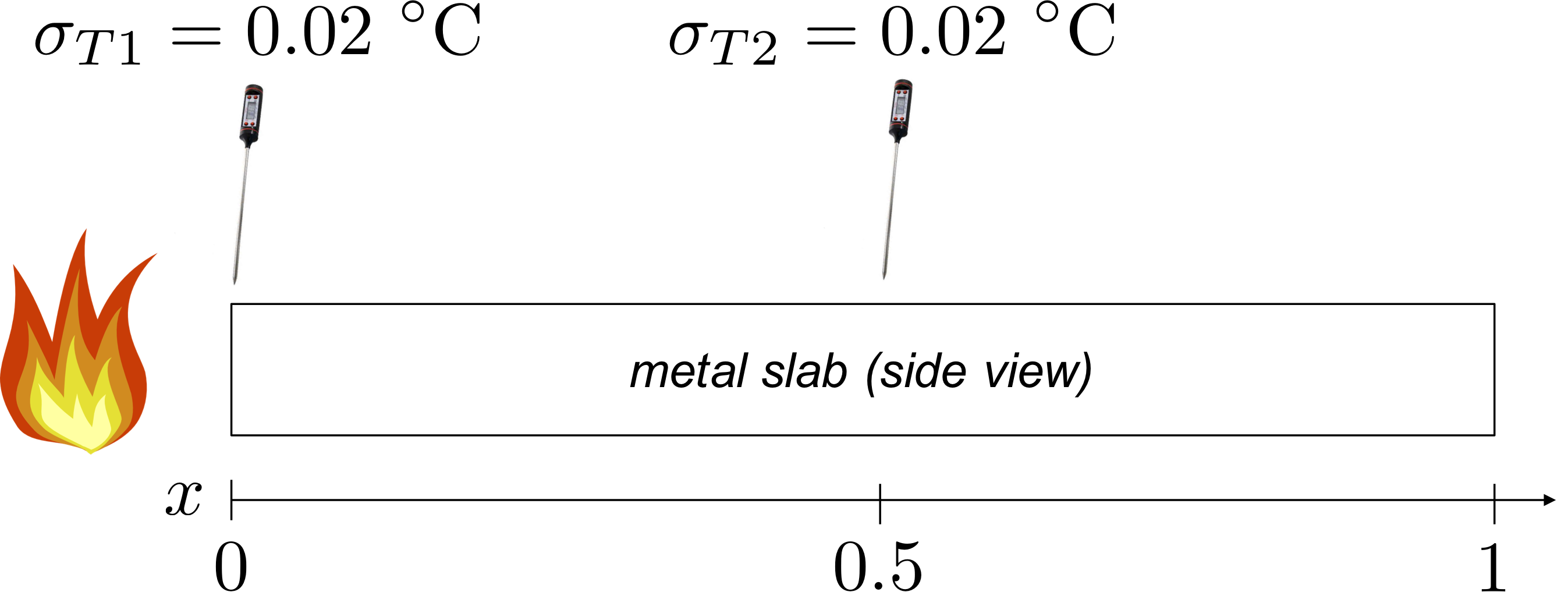
We now have discussed enough of the basics to use finite difference formulas to estimate gradients (derivatives) for experiments. Consider a metal slab heated from one side with two temperature probes:

As time elapses, the temperature throughout the slab increases. The temperature gradient in the slab can be modeled using Fourier’s law of thermal conduction:
where \(k\) is the thermal conductivity of the metal slab. We ultimately want to estimate this material property.
The key challenge in this experiment is estimating the temperature gradient, \(\frac{\partial T}{\partial x}\). To accomplish this, the metal slab has been equipped with two temperature probes, one located at \(x=0\) (probe 1) and another located at \(x=0.5\) (probe 2), as shown in the figure above. These two thermocouples have an absolute precision (\(\sigma_{T1}\), \(\sigma_{T2}\)) of 0.02 \(^\circ{}\)C.
Using the measurements from probes 1 and 2, we can estimate the temperature gradient using a finite difference formula:
5.3.2. Algorithm (Truncation) Error#
Class Activity
With a partner, compute the algorithm (truncation) error using this finite difference formula to approximate the thermal gradient and store the expression in algo_error.
Hint: Start with a Taylor series expansion:
where \(l\) is a length on the slab between 0 and \(h\) such that this formula is exact. Let’s assume that \(\frac{\partial^2 T}{\partial x^2} \approx 4 ~^\circ\)C / unit length\(^2\) and is constant along the slab. With this assumption, \(l\) does not really matter.
# Add your solution here
5.3.3. Random Error#
In a few notebooks, we will formally study probably theory and properties of random variables. If we assume the random errors associated with the temperature probes are independent, we will see soon that the random error in the temperature difference \(\left. T \right|_{x=0.5} - \left. T \right|_{x=0}\) is:
Class Activity
With a partner, compute the random error using the finite difference formula to approximate the thermal gradient. Store the expression in random_error.
# Add your solution here
5.3.4. Optimal Location#
Class Activity
Imagine we can move probe 2 from \(h=0.5\) to another location. With a partner, determine the optimal location such that the truncation error and random error are the same order of magnitude.
Hints: The optimal location is approximated when the truncation error and random error are the same order of magnitude. Modify your expressions for algorithm error and random error from above to depend on \(h\), then set them equal, and finally solve for \(h\). This is the optimal location.
# Add your solution here
5.3.5. Visualize the Results#
Class Activity
Plot your expression of the absolute value of random error and truncation error. Does this trade-off remind you of plots from the previous two notebooks?
# Add your solution here

