7.8. Explicit Range Kutta Method#

Reference: Chapter 17 in Computational Nuclear Engineering and Radiological Science Using Python, R. McClarren (2018).

7.8.1. Learning Objectives#

After studying this notebook, completing the activties, and attending class, you should be able to:

Compare Runge-Kutta to the other three methods.
Error convergence rate
Stability (how does this relate to explicit versus implicit?)
Ease to implement, computational expense (how does this relate to explicit versus implicit?)

# import libraries
import numpy as np
import matplotlib.pyplot as plt
from matplotlib.patches import Polygon
import scipy.integrate as integrate

7.8.2. Fourth-order (Explicit) Runge-Kutta Method#

There is one more method that we need to consider at this point. It is an explicit method called a Runge-Kutta method. The particular one we will learn is fourth-order accurate in \(\Delta t\). That means that if we decrease \(\Delta t\) by a factor of 2, the error will decrease by a factor of \(2^4=16\). The method can be written as

\[y^{n+1} = y^n + \frac{1}{6}\left(\Delta y_1 + 2 \Delta y_2 + 2 \Delta y_3 + \Delta y_4\right),\]

where

\[\Delta y_1 = \Delta t f(y^n, t^n),\]

\[\Delta y_2 = \Delta t f\left(y^n + \frac{\Delta y_1}{2},t^n + \frac{\Delta t}{2}\right),\]

\[\Delta y_3 = \Delta t f\left(y^n + \frac{\Delta y_2}{2},t^n + \frac{\Delta t}{2}\right),\]

\[\Delta y_4 = \Delta t f\left(y^n + \Delta y_3,t^n + \Delta t\right).\]

To get fourth-order accuracy, this method takes a different approach to integrating the right-hand side of the ODE. Basically it makes several projections forward and combines them in such a way that the errors below \(\Delta t^4\) cancel out.

Additional details with a nice illustration: https://en.wikipedia.org/wiki/Runge–Kutta_methods

Implementing this method is not difficult either.

Class Activity

Discuss the code below with a partner. Be prepared to share one question or observation with the class after 3 minutes.

Home Activity

Complete the function below. Hint: You should write two lines of Python code. The first line should calculate dy3 and the second line should calculate dy4.

def RK4(f,y0,Delta_t,numsteps):
    """Perform numsteps of the 4th order Runge-Kutta method starting at y0
    of the ODE y'(t) = f(y,t)
    Args:
        f: function to integrate takes arguments y,t
        y0: initial condition
        Delta_t: time step size
        numsteps: number of time steps
        
    Returns:
        a numpy array of the times and a numpy
        array of the solution at those times
    """
    numsteps = int(numsteps)
    y = np.zeros(numsteps+1)
    t = np.arange(numsteps+1)*Delta_t
    y[0] = y0
    for n in range(1,numsteps+1):
        dy1 = Delta_t * f(y[n-1], t[n-1])
        dy2 = Delta_t * f(y[n-1] + 0.5*dy1, t[n-1] + 0.5*Delta_t)
        # Add your solution here
        y[n] = y[n-1] + 1.0/6.0*(dy1 + 2.0*dy2 + 2.0*dy3 + dy4)
    return t, y

We’ll test this on our problem with a simple exponential solution.

RHS = lambda y,t: -y
Delta_t = 0.1
t_final = 0.4
t,y = RK4(RHS,1,Delta_t,t_final/Delta_t)
plt.plot(t,y,'-',label="Runge-Kutta (4th order)",color="purple",marker="*",markersize=4)
t_fine = np.linspace(0,t_final,100)
plt.plot(t_fine,np.exp(-t_fine),label="Exact Solution",color="black")
plt.xlabel("t")
plt.ylabel("y(t)")
plt.legend()
plt.title("Solution with $\Delta t$ = " + str(Delta_t))
plt.show()
for i in range(len(t)):
    print("Time",round(t[i],1)," : ",y[i])

../../_images/Explicit-Runge-Kutta_9_0.png

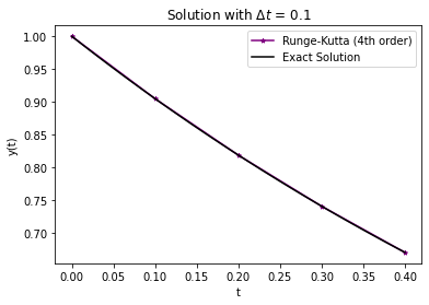
Time 0.0  :  1.0
Time 0.1  :  0.9048375
Time 0.2  :  0.8187309014062499
Time 0.3  :  0.7408184220011776
Time 0.4  :  0.6703202889174906

Your function in the last home activity works if it computes the following values:

t	y
0.0	1.0
0.1	0.9048375
0.2	0.8187309
0.3	0.74081842
0.4	0.67032029

# Removed autograder test. You may delete this cell.

Run the cell below to plot Range-Kutta with different step sizes.

RHS = lambda y,t: -y
Delta_t = np.array([1.0,.5,.25,.125,.0625,.0625/2])
t_final = 2
error = np.zeros(Delta_t.size)
t_fine = np.linspace(0,t_final,100)
count = 0
for d in Delta_t:
    t,y = RK4(RHS,1,d,t_final/d)
    plt.plot(t,y,label="$\Delta t$ = " + str(d))
    error[count] = np.linalg.norm((y-np.exp(-t)))/np.sqrt(t_final/d)
    count += 1
plt.plot(t_fine,np.exp(-t_fine),linewidth=3,color="black",label="Exact Solution")
plt.xlabel("t")
plt.ylabel("y(t)")
plt.legend()
plt.title("Solution with $\Delta t$ = " + str(Delta_t))
plt.show()
plt.loglog(Delta_t,error,'o-',color="purple")
slope = (np.log(error[-1]) - np.log(error[-2]))/(np.log(Delta_t[-1])- np.log(Delta_t[-2]))
plt.title("Slope of Error is " + str(slope))
plt.xlabel("$\Delta t$")
plt.ylabel("Norm of Error")
plt.show()

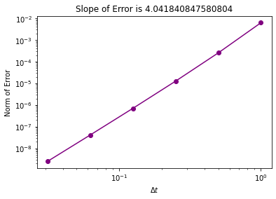
../../_images/Explicit-Runge-Kutta_13_0.png

../../_images/Explicit-Runge-Kutta_13_1.png

Yes, we do indeed get 4th order convergence, as the name fourth-order Runge-Kutta suggests.

We can also try this on our more complicated problem.

First run the cell below with Crank-Nicolson to use in the following example.

def inexact_newton(f,x0,delta = 1.0e-7, epsilon=1.0e-6, LOUD=False):
    """Find the root of the function f via Newton-Raphson method
    Args:
        f: function to find root of
        x0: initial guess
        delta: finite difference parameter
        epsilon: tolerance
        
    Returns:
        estimate of root
    """
    x = x0
    if (LOUD):
        print("x0 =",x0)
    iterations = 0
    while (np.fabs(f(x)) > epsilon):
        fx = f(x)
        fxdelta = f(x+delta)
        slope = (fxdelta - fx)/delta
        if (LOUD):
            print("x_",iterations+1,"=",x,"-",fx,"/",slope,"=",x - fx/slope)
        x = x - fx/slope
        iterations += 1
    if LOUD:
        print("It took",iterations,"iterations")
    return x #return estimate of root

def crank_nicolson(f,y0,Delta_t,numsteps, LOUD=False):
    """Perform numsteps of the backward euler method starting at y0
    of the ODE y'(t) = f(y,t)
    Args:
        f: function to integrate takes arguments y,t
        y0: initial condition
        Delta_t: time step size
        numsteps: number of time steps
        
    Returns:
        a numpy array of the times and a numpy
        array of the solution at those times
    """
    numsteps = int(numsteps)
    y = np.zeros(numsteps+1)
    t = np.arange(numsteps+1)*Delta_t
    y[0] = y0
    for n in range(1,numsteps+1):
        if LOUD:
            print("\nt =",t[n])
            
        # setup nonlinear system
        solve_func = lambda u: u-y[n-1] - 0.5*Delta_t*(f(u,t[n])
                                                       + f(y[n-1],t[n-1]))
        # solve nonlinear system
        y[n] = inexact_newton(solve_func,y[n-1])
        
        if LOUD:
            print("y =",y[n])
    return t, y

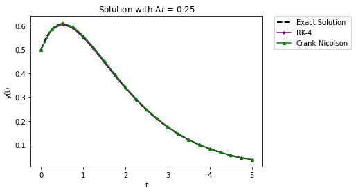
Run the following cell to compare RK-4 and Crank-Nicolson with a step size of 0.25.

RHS = lambda y,t: (1/(t+0.5)-1)*y
exact_sol = lambda t: (t+0.5)*np.exp(-t)
Delta_t = 0.25
t_final = 5
t_fine = np.linspace(0,t_final,100)

plt.plot(t_fine,exact_sol(t_fine),label="Exact Solution",
         linewidth = 2,linestyle="--",color="black")

t,y = RK4(RHS,0.5,Delta_t,t_final/Delta_t)
plt.plot(t,y,label="RK-4",color="purple",marker="*",markersize=4)

t,y = crank_nicolson(RHS,0.5,Delta_t,t_final/Delta_t)
plt.plot(t,y,label="Crank-Nicolson",color="green",marker="^",markersize=4)
plt.xlabel("t")
plt.ylabel("y(t)")
plt.legend(bbox_to_anchor=(1.05, 1), loc=2, borderaxespad=0.)
plt.title("Solution with $\Delta t$ = " + str(Delta_t))
plt.show()

../../_images/Explicit-Runge-Kutta_18_0.png

Run the following cell to compare RK-4 and Crank-Nicolson with a step size of 0.5.

RHS = lambda y,t: (1/(t+0.5)-1)*y
exact_sol = lambda t: (t+0.5)*np.exp(-t)
Delta_t = 0.5
t_final = 5
t_fine = np.linspace(0,t_final,100)

plt.plot(t_fine,exact_sol(t_fine),label="Exact Solution",
         linewidth = 2,linestyle="--",color="black")

t,y = RK4(RHS,0.5,Delta_t,t_final/Delta_t)
plt.plot(t,y,label="RK-4",color="purple",marker="*",markersize=4)

t,y = crank_nicolson(RHS,0.5,Delta_t,t_final/Delta_t)
plt.plot(t,y,label="Crank-Nicolson",color="green",marker="^",markersize=4)

plt.xlabel("t")
plt.ylabel("y(t)")
plt.legend(bbox_to_anchor=(1.05, 1), loc=2, borderaxespad=0.)
plt.title("Solution with $\Delta t$ = " + str(Delta_t))
plt.show()

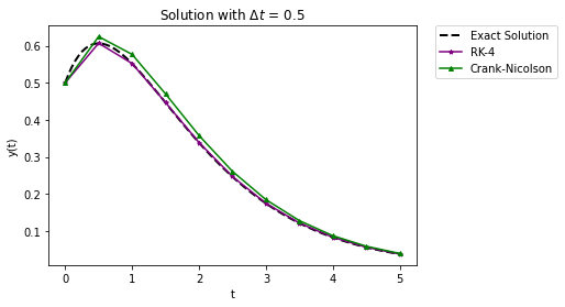
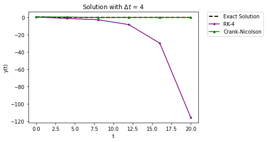
../../_images/Explicit-Runge-Kutta_20_0.png

It also seems to do better that Crank-Nicolson with a large time step, but since it is an explicit method, there are limits: with a large enough time step the solution will oscillate and can be unstable. Below the plot shows a comparison with a larger step size of 4.0.

RHS = lambda y,t: (1/(t+0.5)-1)*y
exact_sol = lambda t: (t+0.5)*np.exp(-t)
Delta_t = 4
t_final = 20
t_fine = np.linspace(0,t_final,100)

plt.plot(t_fine,exact_sol(t_fine),label="Exact Solution",
         linewidth = 2,linestyle="--",color="black")

t,y = RK4(RHS,0.5,Delta_t,t_final/Delta_t)
plt.plot(t,y,'-',label="RK-4",color="purple",marker="*",markersize=4)

t,y = crank_nicolson(RHS,0.5,Delta_t,t_final/Delta_t)
plt.plot(t,y,'-',label="Crank-Nicolson",color="green",marker="^",markersize=4)

plt.xlabel("t")
plt.ylabel("y(t)")
plt.legend(bbox_to_anchor=(1.05, 1), loc=2, borderaxespad=0.)
plt.title("Solution with $\Delta t$ = " + str(Delta_t))
plt.show()

../../_images/Explicit-Runge-Kutta_22_0.png

Class Activity

Discuss with a partner: Why should you use RK4? When should you use Crank-Nicolson?

Data and Computing for Chemical Engineers

Explicit Range Kutta Method

Contents

7.8. Explicit Range Kutta Method#

7.8.1. Learning Objectives#

7.8.2. Fourth-order (Explicit) Runge-Kutta Method#