Algorithms Homework 4#
Assigment Overview: This assignment implements a basic interior point method for nonlinear programs with equality constraints and bounds.
Tips and Tricks#
Background#
Recall, the step for a primal-dual interior point method is defined by the following system of linear equations (Eq. 6.56 in Biegler, 2010):
Alternatively, the step for the dual variables for the bounds can be recommed for this system (Eq. 6.57 in Biegler, 2010):
And then computed using the solution to the linear system (Eq. 6.58 in Biegler, 2010):
Finally, inertia correction and regularization can be applied to ensure reliable calculation of the Newton step (Eq. 6.59 in Biegler, 2010):
Problem Formulation#
Consider the following nonlinear program:
where \(x \in \mathbb{R}^{n}\), \(f(x): \mathbb{R}^{n} \rightarrow \mathbb{R}\), \(c(x): \mathbb{R}^{n} \rightarrow \mathbb{R}^{m}\) and \(|\mathcal{I} |\) = \(r\) (i.e., there are \(r\) variables with a lower bound and \(r \leq n\)). This is an extension of (6.48) in Biegler (2010).
This has the corresponding log-barrier approximation:
which is an extension of (6.49) in Biegler (2010).
Let the \(n \times r\) matrix \(G\) encode which variables are bounded. If variable \(i\) corresponds to the \(j\)th bound, then \(G_{i,j} = 1\) and otherwise \(G_{i,j} = 0\).
\(G\) is assembled as follows:
Initialize \(G\) as the zero matrix
Loop over \(k=1\) to \(k=|\mathcal{I}\)
Extract the index \(i\) corresponding to the element \(\mathcal{I}_k\)
Set \(G_{i,k} = 1\)
Notice that \(G\) is the gradient of \(x \geq 0\). \(G^T G = I\) but the converse does not hold unless \(r = n\).
Reformulation Example#
Start with:
Add slack variable \(x_3\) and convert the inequality constraint to an equality constraint and bound:
Now assemble \(G\):
Primal Dual Optimality Conditions#
Next we extend (6.51) in Biegler (2010):
We now extend (6.56) in Biegler (2010):
where \(U^k = \mathrm{diag}\{u^k\}\) and \(W^k = \nabla_{xx} L(x^k,v^k)\). Notice that \(W^k\) does NOT include a contribution from the barrier term:
We can verify that \(W^k\) does not include \(\hat{X}\) by showing that the KKT system above is a Newton step to solve the nonlinear system for the primal dual conditions.
The Newton step can be simplified, similar to (6.57) and (6.58) in Biegler (2010):
and
where
and
Notice that the equation for \(\du\) simplifies by substituting \(G^T G = I\):
Finally, inertia correction can be applied to simplified KKT step similar to (6.59) in Biegler (2010).
Basic Interior Point Method for Inequality and Equality Constraint NLPs#
Implement a basic interior point method for inequality and equality constrained nonlinear programs. See pg. 154 – 155 in Biegler (2010). You may skip the line search, i.e., always take a full step.
Pseudocode#
Write detailed pseudocode on paper or a whiteboard. Scan/take a photo and turn in.
Python Implementation#
Implement in Python. Hints: Reuse code from Algorithm 5.2 example.
### Load Python libraries

import sys
if "google.colab" in sys.modules:
    !wget "https://raw.githubusercontent.com/ndcbe/optimization/main/notebooks/helper.py"
    import helper
    # helper.easy_install() # We do NOT need Pyomo for this assignment
else:
    sys.path.insert(0, '../../../optimization/notebooks/')
    import helper
helper.set_plotting_style() # But we do want the nice plots

import numpy as np
from scipy import linalg


### Define helper functions
## Check is element of array is NaN
def check_nan(A):
    return np.sum(np.isnan(A))

## Calculate gradient with central finite difference
def my_grad_approx(x,f,eps1,verbose=False):
    '''
    Calculate gradient of function f using central difference formula

    Inputs:
        x - point for which to evaluate gradient
        f - function to consider
        eps1 - perturbation size

    Outputs:
        grad - gradient (vector)
    '''

    n = len(x)
    grad = np.zeros(n)

    if(verbose):
        print("***** my_grad_approx at x = ",x,"*****")

    for i in range(0,n):

        # Create vector of zeros except eps in position i
        e = np.zeros(n)
        e[i] = eps1

        # Finite difference formula
        my_f_plus = f(x + e)
        my_f_minus = f(x - e)

        # Diagnostics
        if(verbose):
            print("e[",i,"] = ",e)
            print("f(x + e[",i,"]) = ",my_f_plus)
            print("f(x - e[",i,"]) = ",my_f_minus)


        grad[i] = (my_f_plus - my_f_minus)/(2*eps1)

    if(verbose):
        print("***** Done. ***** \n")

    return grad

## Calculate gradient with central finite difference
def my_jac_approx(x,h,eps1,verbose=False):
    '''
    Calculate Jacobian of function h(x) using central difference formula

    Inputs:
        x - point for which to evaluate gradient
        h - vector-valued function to consider. h(x): R^n --> R^m
        eps1 - perturbation size

    Outputs:
        A - Jacobian (n x m matrix)
    '''

    # Check h(x) at x
    h_x0 = h(x)

    # Extract dimensions
    n = len(x)
    m = len(h_x0)

    # Initialize Jacobian matrix
    A = np.zeros((n,m))

    # Calculate Jacobian by row
    for i in range(0,n):

        # Create vector of zeros except eps in position i
        e = np.zeros(n)
        e[i] = eps1

        # Finite difference formula
        my_h_plus = h(x + e)
        my_h_minus = h(x - e)

        # Diagnostics
        if(verbose):
            print("e[",i,"] = ",e)
            print("h(x + e[",i,"]) = ",my_h_plus)
            print("h(x - e[",i,"]) = ",my_h_minus)


        A[i,:] = (my_h_plus - my_h_minus)/(2*eps1)

    if(verbose):
        print("***** Done. ***** \n")

    return A

## Calculate Hessian using central finite difference
def my_hes_approx(x,grad,eps2):
    '''
    Calculate gradient of function my_f using central difference formula and my_grad

    Inputs:
        x - point for which to evaluate gradient
        grad - function to calculate the gradient
        eps2 - perturbation size (for Hessian NOT gradient approximation)

    Outputs:
        H - Hessian (matrix)
    '''

    n = len(x)
    H = np.zeros([n,n])

    for i in range(0,n):
        # Create vector of zeros except eps in position i
        e = np.zeros(n)
        e[i] = eps2

        # Evaluate gradient twice
        grad_plus = grad(x + e)
        grad_minus = grad(x - e)

        # Notice we are building the Hessian by column (or row)
        H[:,i] = (grad_plus - grad_minus)/(2*eps2)

    return H

## Linear algebra calculation
def xxT(u):
    '''
    Calculates u*u.T to circumvent limitation with SciPy

    Arguments:
    u - numpy 1D array

    Returns:
    u*u.T

    Assume u is a nx1 vector.
    Recall: NumPy does not distinguish between row or column vectors

    u.dot(u) returns a scalar. This functon returns an nxn matrix.
    '''

    n = len(u)
    A = np.zeros([n,n])
    for i in range(0,n):
        for j in range(0,n):
            A[i,j] = u[i]*u[j]

    return A

## Analyze Hessian
def analyze_hes(B):
    print(B,"\n")

    l = linalg.eigvals(B)
    print("Eigenvalues: ",l,"\n")
## Assemble KKT matrix (equality constrained only)
def assemble_check_KKT(W,Sk,A,deltaA,deltaW,verbose):

    # Add your solution here

    return KKT,inertia_correct,pos_ev,neg_ev,zero_ev
def barrier_subproblem(x0,v0,u0,calc_f,calc_c,var_bounds,mu,eps,max_iter=100,verbose=False):
    '''
    Basic Full Space Newton Method for Solving Barrier Subproblem Constrained NLP

    Input:
        x0 - starting point (vector)
        calc_f - function to calculate objective (returns scalar)
        calc_c - function to calculate constraints (returns vector)
        var_bounds - list of indicies for variables with lower bound
        mu - barrier penalty
        eps - tolerance for termination

    Histories (stored for debugging):
        x - history of steps (primal variables)
        v - history of steps (duals for constraints)
        u - history of steps (duals for bounds)
        f - history of objective evaluations
        c - history of constraint evaluations
        df - history of objective gradients
        dL - history of Lagrange function gradients
        A - history of constraint Jacobians
        W - history of Lagrange Hessians
        S - history of sigma matrix

    Outputs:
        x - final value for primal variable
        v - final value for constraint duals
        u - final value for bound duals

    Notes:
        1. For simplicity, central finite difference is used
           for all gradient calculations.
    '''

    ### Specifics for Algorithm 5.2
    # Tuning parameters
    delta_bar_W_min = 1E-20
    delta_bar_W_0 = 1E-4
    delta_bar_W_max = 1E40
    delta_bar_A = 1E-8
    kappa_u = 8
    kappa_l = 1/3

    # Declare iteration histories as empty lists
    x = []
    v = []
    u = []
    f = []
    L = []
    c = []
    df = []
    dL = []
    A = []
    W = []

    # Add your solution here
def interior_point(x0,calc_f,calc_c,var_bounds,max_iter=20):


    # Add your solution here

    return x, v, u, mu, E
Test Problems#
Problem 1: Convex#
f = lambda x: x[0] + 2*x[1]
c = lambda x: (x[0] + x[1] - 1)*np.ones(1)

# Indices of variables with lower bound of zero
vb = [1]

x0 = np.ones(2)
u0 = np.ones(1)
v0 = np.ones(1)

x_, v_, u_, E_ = barrier_subproblem(x0,v0,u0,f,c,vb,1E-1,1E-10,verbose=False)
Iter. 	f(x) 		||c(x)|| 	E 		||dx|| 		||dv|| 		||du|| 		delta_A 	delta_W
0   	 3.0000e+00 	1.0000e+00 	 2.00e+00 	 9.06e-01 	 2.00e+00 	 3.56e-04 	 0.00e+00 	 0.00e+00
1   	 1.0996e+00 	1.3978e-10 	 3.20e-04 	 5.03e-04 	 1.78e-04 	 3.56e-04 	 0.00e+00 	 0.00e+00
2   	 1.1000e+00 	3.9524e-14 	 1.26e-07 	 1.70e-07 	 3.94e-08 	 5.91e-08 	 0.00e+00 	 0.00e+00
3   	 1.1000e+00 	0.0000e+00 	 6.87e-11 	 1.48e-11 	 1.11e-10 	 1.04e-10 	 0.00e+00 	 0.00e+00
Problem 2: Convex#
f = lambda x: x[0] + 2*x[1]
c = lambda x: (x[0] + x[1] - 1)*np.ones(1)

# Indices of variables with lower bound of zero
vb = [1]

x0 = np.ones(2)
#u0 = np.ones(1)
#v0 = np.ones(1)

# x_, v_, u_, E_ = barrier_subproblem(x0,v0,u0,f,c,vb,1E-1,1E-10,verbose=False)

x, v, u, mu, E = interior_point(x0,f,c,vb)
*** Barrier Subproblem  0  ***
mu =  10.0
Iter. 	f(x) 		||c(x)|| 	E 		||dx|| 		||dv|| 		||du|| 		delta_A 	delta_W
0   	 3.0000e+00 	1.0000e+00 	 9.00e+00 	 1.35e+01 	 2.00e+00 	 8.45e-03 	 0.00e+00 	 0.00e+00

*** Barrier Subproblem  1  ***
mu =  2.0
Iter. 	f(x) 		||c(x)|| 	E 		||dx|| 		||dv|| 		||du|| 		delta_A 	delta_W
0   	 1.1008e+01 	1.3978e-10 	 7.92e+00 	 1.14e+01 	 4.22e-03 	 8.45e-03 	 0.00e+00 	 0.00e+00

*** Barrier Subproblem  2  ***
mu =  0.4
Iter. 	f(x) 		||c(x)|| 	E 		||dx|| 		||dv|| 		||du|| 		delta_A 	delta_W
0   	 2.9318e+00 	0.0000e+00 	 1.53e+00 	 2.17e+00 	 1.70e-04 	 3.40e-04 	 0.00e+00 	 0.00e+00

*** Barrier Subproblem  3  ***
mu =  0.08000000000000002
Iter. 	f(x) 		||c(x)|| 	E 		||dx|| 		||dv|| 		||du|| 		delta_A 	delta_W
0   	 1.3993e+00 	2.5520e-10 	 3.19e-01 	 4.51e-01 	 1.70e-04 	 3.40e-04 	 0.00e+00 	 0.00e+00

*** Barrier Subproblem  4  ***
mu =  0.016000000000000004
Iter. 	f(x) 		||c(x)|| 	E 		||dx|| 		||dv|| 		||du|| 		delta_A 	delta_W
0   	 1.0801e+00 	5.3163e-11 	 6.41e-02 	 9.07e-02 	 1.07e-05 	 1.78e-05 	 0.00e+00 	 0.00e+00

*** Barrier Subproblem  5  ***
mu =  0.0020238577025077633
Iter. 	f(x) 		||c(x)|| 	E 		||dx|| 		||dv|| 		||du|| 		delta_A 	delta_W
0   	 1.0160e+00 	0.0000e+00 	 1.40e-02 	 1.98e-02 	 1.15e-05 	 1.86e-05 	 0.00e+00 	 0.00e+00

*** Barrier Subproblem  6  ***
mu =  9.104790579399288e-05
Iter. 	f(x) 		||c(x)|| 	E 		||dx|| 		||dv|| 		||du|| 		delta_A 	delta_W
0   	 1.0020e+00 	7.7571e-13 	 1.93e-03 	 2.73e-03 	 7.76e-07 	 8.83e-07 	 0.00e+00 	 0.00e+00
1   	 1.0001e+00 	0.0000e+00 	 1.07e-07 	 2.43e-09 	 0.00e+00 	 1.07e-07 	 0.00e+00 	 0.00e+00

*** Barrier Subproblem  7  ***
mu =  8.687702517211205e-07
Iter. 	f(x) 		||c(x)|| 	E 		||dx|| 		||dv|| 		||du|| 		delta_A 	delta_W
0   	 1.0001e+00 	0.0000e+00 	 9.02e-05 	 1.28e-04 	 1.11e-10 	 5.12e-09 	 0.00e+00 	 0.00e+00
1   	 1.0000e+00 	9.9920e-15 	 4.95e-09 	 6.52e-13 	 3.88e-17 	 4.95e-09 	 0.00e+00 	 0.00e+00
import matplotlib.pyplot as plt
def plot_results(x,u,v,mu,E):
''' Plot results of interior point method
Inputs:
x - primal variables
u - dual variables for lower bounds
v - dual variables for equality constraints
mu - barrier penalty
E - error
Outputs:
None
Other:
Plots are generated.
'''
# number of iterations
N = len(x)
# iteration
iters = range(0,N)
plt.figure
for i in range(0,len(x0)):
plt.plot(iters,[x[j][i] for j in range(0,N)],label="$x_{"+str(i)+"}$")
plt.xlabel("Iteration")
plt.ylabel("Primal Variables")
plt.legend()
plt.show()
plt.figure
for i in range(0,len(u[0])):
plt.plot(iters,[u[j][i] for j in range(0,N)],label="$u_{"+str(i)+"}$")
for i in range(0,len(v[0])):
plt.plot(iters,[v[j][i] for j in range(0,N)],label="$v_{"+str(i)+"}$")
plt.xlabel("Iteration")
plt.ylabel("Dual Variables")
plt.legend()
plt.show()
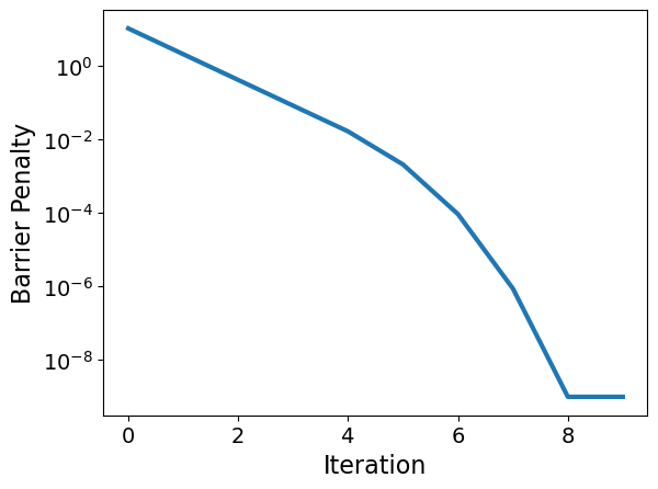
plt.figure
plt.semilogy(iters,mu)
plt.xlabel("Iteration")
plt.ylabel("Barrier Penalty")
plt.show()
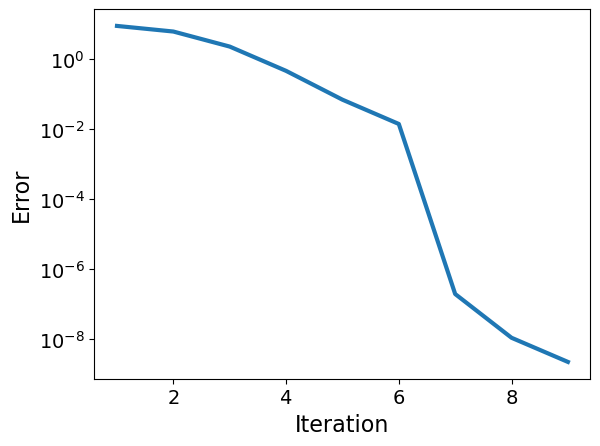
plt.figure
plt.semilogy(range(1,N),E)
plt.xlabel("Iteration")
plt.ylabel("Error")
plt.show()
plot_results(x,u,v,mu,E)
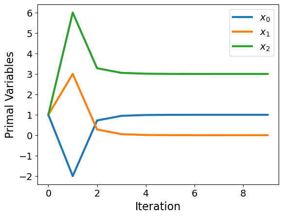
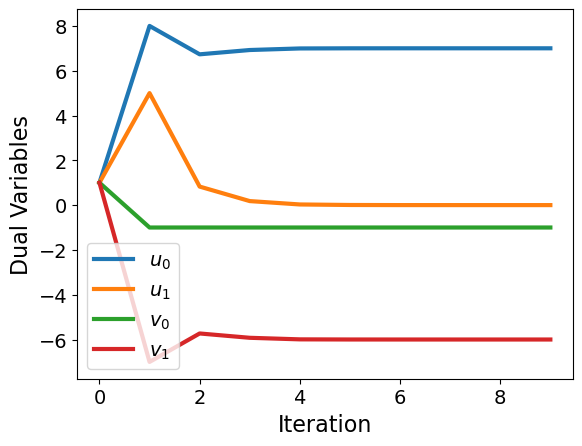
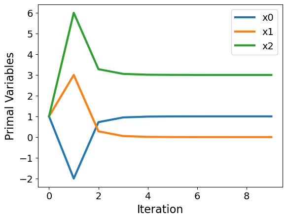
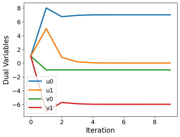
Problem 3: Nonconvex#
f = lambda x: x[0] + 2*x[1] + x[2]**2

def c(x):
    rhs = np.zeros(2)
    rhs[0] = x[0] + x[1] - 1
    rhs[1] = x[2] - x[1] - 3
    return rhs

# Indices of variables with lower bound of zero
vb = [1,2]

x0 = np.ones(3)
u0 = np.ones(2)
v0 = np.ones(2)

## Test barrier subproblem
# xtest, vtest, utest, Etest = barrier_subproblem(x0,v0,u0,f,c,vb,1E-1,1E-10,max_iter=10,verbose=True)

##
x, v, u, mu, E = interior_point(x0,f,c,vb)
*** Barrier Subproblem  0  ***
mu =  10.0
Iter. 	f(x) 		||c(x)|| 	E 		||dx|| 		||dv|| 		||du|| 		delta_A 	delta_W
0   	 4.0000e+00 	3.1623e+00 	 9.00e+00 	 6.17e+00 	 8.25e+00 	 8.06e+00 	 0.00e+00 	 0.00e+00

*** Barrier Subproblem  1  ***
mu =  2.0
Iter. 	f(x) 		||c(x)|| 	E 		||dx|| 		||dv|| 		||du|| 		delta_A 	delta_W
0   	 4.0013e+01 	4.4202e-10 	 2.80e+01 	 3.79e+00 	 1.52e+00 	 3.22e+00 	 0.00e+00 	 0.00e+00
1   	 1.6354e+01 	8.8818e-16 	 6.22e+00 	 9.26e-01 	 2.48e-01 	 1.35e+00 	 0.00e+00 	 0.00e+00

*** Barrier Subproblem  2  ***
mu =  0.4
Iter. 	f(x) 		||c(x)|| 	E 		||dx|| 		||dv|| 		||du|| 		delta_A 	delta_W
0   	 1.2028e+01 	5.9365e-11 	 2.31e+00 	 3.93e-01 	 1.93e-01 	 6.75e-01 	 0.00e+00 	 0.00e+00

*** Barrier Subproblem  3  ***
mu =  0.08000000000000002
Iter. 	f(x) 		||c(x)|| 	E 		||dx|| 		||dv|| 		||du|| 		delta_A 	delta_W
0   	 1.0363e+01 	5.0425e-11 	 4.67e-01 	 7.00e-02 	 6.98e-02 	 1.66e-01 	 0.00e+00 	 0.00e+00

*** Barrier Subproblem  4  ***
mu =  0.016000000000000004
Iter. 	f(x) 		||c(x)|| 	E 		||dx|| 		||dv|| 		||du|| 		delta_A 	delta_W
0   	 1.0077e+01 	0.0000e+00 	 7.01e-02 	 1.52e-02 	 5.73e-03 	 2.39e-02 	 0.00e+00 	 0.00e+00

*** Barrier Subproblem  5  ***
mu =  0.0020238577025077633
Iter. 	f(x) 		||c(x)|| 	E 		||dx|| 		||dv|| 		||du|| 		delta_A 	delta_W
0   	 1.0016e+01 	2.1737e-12 	 1.42e-02 	 3.45e-03 	 7.37e-04 	 4.77e-03 	 0.00e+00 	 0.00e+00

*** Barrier Subproblem  6  ***
mu =  9.104790579399288e-05
Iter. 	f(x) 		||c(x)|| 	E 		||dx|| 		||dv|| 		||du|| 		delta_A 	delta_W
0   	 1.0002e+01 	4.4187e-13 	 1.94e-03 	 4.78e-04 	 9.60e-05 	 6.55e-04 	 0.00e+00 	 0.00e+00
1   	 1.0000e+01 	1.5321e-14 	 1.95e-07 	 6.73e-09 	 1.77e-07 	 1.43e-07 	 0.00e+00 	 0.00e+00

*** Barrier Subproblem  7  ***
mu =  8.687702517211205e-07
Iter. 	f(x) 		||c(x)|| 	E 		||dx|| 		||dv|| 		||du|| 		delta_A 	delta_W
0   	 1.0000e+01 	0.0000e+00 	 9.02e-05 	 2.23e-05 	 4.30e-06 	 3.04e-05 	 0.00e+00 	 0.00e+00
1   	 1.0000e+01 	1.4433e-15 	 1.10e-08 	 1.38e-11 	 1.24e-08 	 2.28e-08 	 0.00e+00 	 0.00e+00

*** Barrier Subproblem  8  ***
mu =  1e-09
Iter. 	f(x) 		||c(x)|| 	E 		||dx|| 		||dv|| 		||du|| 		delta_A 	delta_W
0   	 1.0000e+01 	0.0000e+00 	 8.68e-07 	 2.15e-07 	 4.04e-08 	 2.92e-07 	 0.00e+00 	 0.00e+00
1   	 1.0000e+01 	4.4409e-16 	 2.24e-09 	 1.05e-15 	 1.69e-09 	 4.54e-09 	 0.00e+00 	 0.00e+00
plot_results(x,u,v,mu,E)