4.3. Advanced Topics in Stochastic Programming

This notebook contains advanced topics for optimization under uncertainty.

4.3.1. Sample Average Approximation

Sample average approximation (SAA) method is an approach for solving stochastic optimization problems by Monte Carlo simulation. It approximates the expected objective function of the stochastic problem by a sample average estimate derived from a random sample. The resulting sample average approximation problem is then solved by deterministic optimization techniques.

Consider a stochastic program in the following form:

\(z = \inf \int_{\Xi} g(x,\xi) P(d\xi)\)

The optimal solution \(x^*\) will have optimal value \(z^*\). SAA consider a sample \({\xi^i}\) of independent observations of \(\xi\):

\(z^{\nu} = \inf \frac{1}{\nu} \sum_{i=1}^{\nu} g(x,\xi^i)\)

Where \(x^{\nu}\) is the random vector of solutions with independent random samples, \(\xi^i\), \(i=1,...,\nu\).

4.3.2. Sparse Grids (Worst Case)

Instead of Monte carlo sampling, sparse grids can be used to obtain efficient characterizations of the integrals in stochastic programs. Many computational problems are solved on full grids. While this is feasible if the dimentionality \(d\) of the problem is low, 2 or 3, full grids become very expensive when facing a higher dimentional problem \(d>4\). This is due to the curse of dimensionality, which states that the complexity of full grids grows exponentially with \(d\).

Sparse grids defeat the curse of dimentionality and allow the solution of the problems with much smaller effort. It is constructed by extending one-dimensional quadrature rules to higher dimensions. Gaussian quadrature rule is one of these rules to approximate the definite integral of a function. It is usually a weighted sum of function values at specified points within the domain of integration, stated as:

\(\int f(x)dx \approx \sum_{i=1}^{n} \omega_i f(x_i) \)

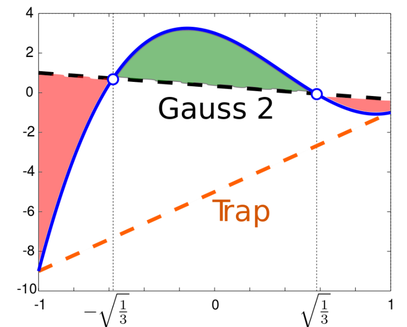
Comparison between 2-point Gaussian and trapezoidal quadrature. For the polynomial:

\(y(x) = 7x^3-8x^2-3x+3\)

whose integral in [-1,1] is \(\frac{2}{3}\).

The trapezoidal rule returns the integral of the orange dashed line:

\(y(-1)+y(1) = -10\)

The 2-point Gaussian quadrature returns the integral of the black dashed curve, equal to:

\(y(-\sqrt{\frac{1}{3}}) + y(\sqrt{\frac{1}{3}}) = \frac{2}{3}\)

Figure from [1]

import Tasmanian
import numpy as np
import matplotlib.pyplot as plt

# define bounds for integration
UB = 1
LB = -1

# function
y = lambda x: 7*x**3-8*x**2-3*x+3

# integrated function 
int_y = lambda x: 1.75*x**4-8/3*x**3-1.5*x**2+3*x

# real area 
real_S = int_y(UB) - int_y(LB)
print('The area:', real_S)

# area calculated by trapezoidal rule
trap_S = (y(UB)+y(LB))*(UB-LB)/2
print('The area calculated by trapezoidal rule:', trap_S)

# generate sparse grids
range_p = np.array([[LB,UB]])
grid_p = Tasmanian.SparseGrid()
grid_p.makeGlobalGrid(1,0,1,'level','gauss-legendre')
grid_p.setDomainTransform(range_p)
points_p = grid_p.getPoints()
weights_p = grid_p.getQuadratureWeights()
# area calculated by sparse grids
gauss_S = sum(y(point)*weights_p[i] for i, point in enumerate(points_p))
print('The area calculated by Gauss rule:', gauss_S)

How to choose quadrature rules for sparse grids depends on how the problem is formed. A guidance on how to choose the one dimensional quadrature rule can be found in: https://tasmanian.ornl.gov/documentation/group__SGEnumerates.html#ga145e27d5ae92acdd5f74149c6d4f2ca2

The following example shows several example quadrature rules:

def show_sparse_grids(range_p,dim=2,output=0,depth=5, rule='gauss-legendre'):
    '''
    This function shows the sparse grids generated with different rules
    Arguments:
        range_p: dimension ranges 
        dim: sparse grids dimension
        output: output level
        depth: depth level
        rule: quadrature rules
    Return: 
        None
    Other:
        A figure shows 2D sparse grids
    '''
    grid_p = Tasmanian.SparseGrid()
    grid_p.makeGlobalGrid(dim,output,depth,'level',rule)
    grid_p.setDomainTransform(range_p)
    points_p = grid_p.getPoints()
    weights_p = grid_p.getQuadratureWeights()
    
    for i in range(len(points_p)):
        plt.scatter(points_p[i,0], points_p[i,1])
        plt.title('Sparse girds of '+rule)
    plt.show()
    
range_fix = np.array([[50,220],[300,600]])
show_sparse_grids(range_fix)
show_sparse_grids(range_fix, rule='gauss-hermite')
show_sparse_grids(range_fix, rule='chebyshev')

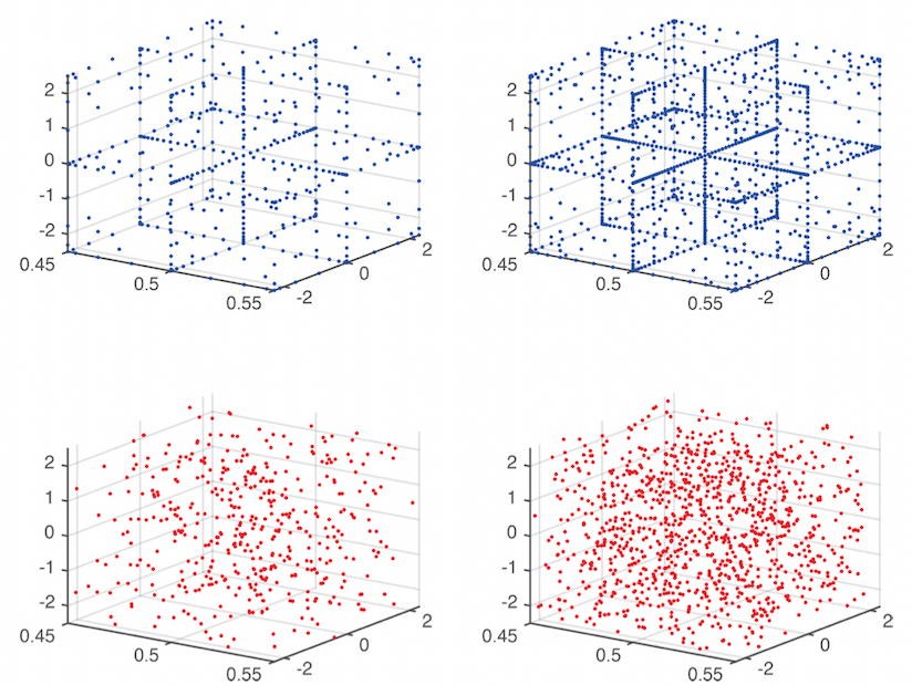
The following figure shows sparse grid on the top, and Monte Carlo samples on the bottom. Left graphs contain 441 scenarios, and the right graphs contain 1073 scenarios. Sparse grids can efficiently cover the domain and lead to higher convergence rates.

Figure from [2]

4.3.3. Reference

Biegler, L.T., 2010. Nonlinear programming: concepts, algorithms, and applications to chemical processes. Society for Industrial and Applied Mathematics.

Birge, J.R. and Louveaux, F., 2011. Introduction to stochastic programming. Springer Science & Business Media.

Figures from:

[1] By Paolostar - Own work, CC BY-SA 4.0, https://commons.wikimedia.org/w/index.php?curid=46820806

[2] Renteria, J.A., Cao, Y., Dowling, A.W. and Zavala, V.M., 2018. Optimal pid controller tuning using stochastic programming techniques. AIChE Journal, 64(8), pp.2997-3010.