Optimization Modeling with Applications

1.2. Optimization Modeling with Applications#

1.2.1. Recommended Reading#

Please review the following book chapters (in order):

Chapter 1 of Biegler (2010) introduces classes of optimization problems motivated by applications.
Chapters 1 and 2 in Hart et al. (2015) provides an overview of Pyomo and optimization modeling.
Chapters 3 and 4 in Hart et al. (2015) describes core Pyomo features through examples.
Chapter 7 in Hart et al. (2015) describes special considerations for nonlinear programs.
Chapter 9 in Hart et al. (2015) describes generalized disjunctive programming (logical decisions).
Chapter 10 in Hart et al. (2015) describes stochastic programming (sections 10.1 - 10.4 are most relevant).
Chapter 11 in Hart et al. (2015) describes optimization with differential algebriac equations (DAEs).
Chapter 10 in Biegler (2010) provides mathematical background for DAE-constrained optimization.

pyomo_book

nlp_book

1.2.2. Taxonomy of Optimization Problems#

Reference: Chapter 1 in Biegler (2010).

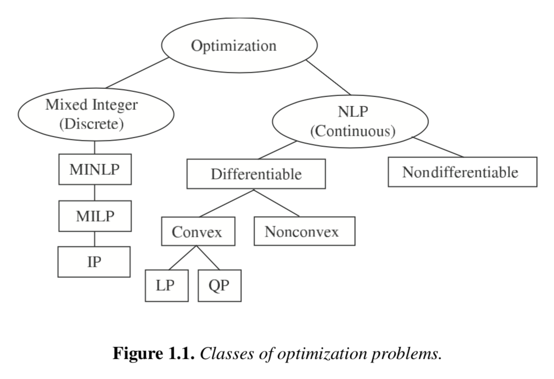
The following chart organizes optimization problems based on key characteristics including variable type (continous versus discrete) and whether the objective and constraints are differentiable. These factors impact which algorithms are best suited for different problems.

taxonomy

1.2.2.1. Linear Programs (LP) / Linear Optimization Problems#

\[\begin{split} \begin{align*} \min_{x} \quad & f^T x & \text{(linear objective)} \\ \text{s.t.} \quad & A \cdot x = b & \text{(linear constraints)} \\ & x^L \leq x \leq x^U & \text{(bounds)} \end{align*} \end{split}\]

Recall, “s.t.” means “subject to”.

How to enforce \(x_1 + x_2 \leq c\) in the above formulation? Convert it to an equality constraint:

\[ x_1 + x_2 = s_1 \]

where \(s_1\) is a slack variable.

1.2.2.2. Quadratic Program (QP)#

\[\begin{split} \begin{align*} \min_{x} \quad & \frac{1}{2} x^T H x + f^T x & \text{(quadratic objective)} \\ \text{s.t.} \quad & A \cdot x = b & \text{(linear constraints)} \\ & x^L \leq x \leq x^U & \text{(bounds)} \end{align*} \end{split}\]

Parameters: \(H\), \(f\), \(A\), \(b\), \(x^L\), \(x^U\)

There are specialized solvers for LP, QP, and other convex optimization problems. We will not focus on these in this class, but instead consider algorithms for general nonlinear programs.

1.2.2.3. Nonlinear Program (NLP)#

\[\begin{split} \begin{align*} \min_{x} \quad & f(x) & \text{(nonlinear objective)} \\ \text{s.t.} \quad & g(x) = 0 & \text{(equality constraints)} \\ & h(x) \leq 0 & \text{(inequality constraints)} \end{align*} \end{split}\]

where \(f(x), g(x), h(x)\) are all nonlinear functions. Bounds can be modeled as inequality constraints.

1.2.2.4. Mixed Integer Nonlinear Programs (MINLP)#

The most general form is:

\[\begin{split} \begin{align*} \min_{x,y} \quad & f(x,y) & \text{(nonlinear objective)} \\ \text{s.t.} \quad & g(x,y) = 0 & \text{(equality constraints)} \\ & h(x,y) \leq 0 & \text{(inequality constraints)} \\ & x \in \mathbb{R}^{n}, ~ y \in \{0,1\}^m \end{align*} \end{split}\]

It is much easier to design algorithms to solve MINLPs with the following structure:

\[\begin{split} \begin{align*} \min_{x,y} \quad & f(x) + g^T y & \text{(nonlinear objective)} \\ \text{s.t.} \quad & A \cdot x + B \cdot y = c & \text{(linear equality constraints)} \\ & g(x) = 0 & \text{(nonlinear equality constraints)} \\ & h(x) \leq 0 & \text{(nonlinear equality constraints)} \\ & x \in \mathbb{R}^{n}, ~ y \in \{0,1\}^m \end{align*} \end{split}\]

where x are continuous and y are discrete (binary) variables. Notice y only enters linearly into the objective and equality constraint.

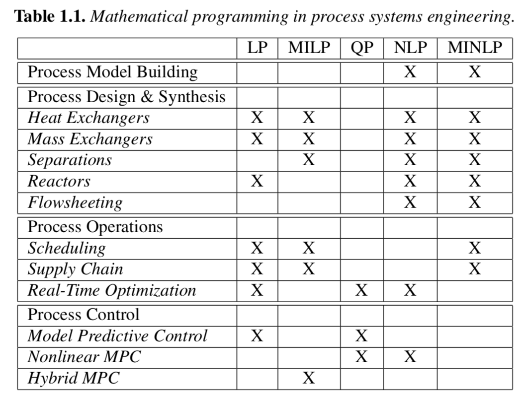
Here are common (chemical) engineering optimization problems organizied by problem type: optimization_examples