3.6. Pyomo.DAE: Racing Example Revisited#
Prepared by: Prof. Alexander Dowling, Molly Dougher (mdoughe6@nd.edu, 2023)
# Install Pyomo and solvers for Google Colab
import sys
if "google.colab" in sys.modules:
    !wget "https://raw.githubusercontent.com/ndcbe/optimization/main/notebooks/helper.py"
    import helper
    helper.easy_install()
else:
    sys.path.insert(0, '../')
    import helper
helper.set_plotting_style()

# import Pyomo library
import pyomo.environ as pyo
import pyomo.dae as dae
import matplotlib.pyplot as plt
3.6.1. Car Example#
Adapted from Pyomo/pyomo
You are a race car driver with a simple goal. Drive distance \(L\) in the minimal amount of time but come to a complete stop at the finish line.
3.6.1.1. Optimal Control Problem Formulation#
Mathematically, you want to solve the following optimal control problem:
where \(a\) is the acceleration/braking (your control variable) and \(R\) is the drag coefficient (parameter).
3.6.1.2. Scale Time#
Let \(t = \tau \cdot t_f\) where \(\tau \in [0,1]\). Thus \(dt = t_f d\tau\). The optimal control problem becomes:
3.6.1.3. Orthogonal Collocation on Finite Elements: Manual Approach#
Here is the “classical”/”old school” way of manually implementing collocation on finite elements with sets.
Indices and Sets
Finite elements: \(i \in \mathcal{I} = \{1,2,...,N_{FE}\}\)
Finite elements (except first): \(\mathcal{I} \setminus 1\)
Internal collocation points: \(j,k \in \mathcal{J} = \{1,2,...,N_{C}\}\)
Parameters
Coefficients in collocation/Runge-Kutta formula: \(a_{j,j}\)
Drag coefficient: \(R\)
Race length: \(L\)
Scaled time for each finite element: \(h_i = \frac{1}{N_{FE}}\)
Variables
Position (internal collocation points): \(x_{i,j}\)
Position (beginning of each finite element): \(\bar{x}_{i}\)
Position derivative (internal collocation points): \(\dot{x}_{i,j}\)
Velocity (internal collocation points): \(v_{i,j}\)
Velocity (beginning of each finite element): \(\bar{v}_{i}\)
Velocity derivative (internal collocation points): \(\dot{v}_{i,j}\)
Time (internal collocation points): \(t_{i,j}\)
Time (beginning of each finite element): \(\bar{t}_{i}\)
Acceleration (control degrees of freedom): \(u_i\)
Objective and Constraints
import pyomo.environ as pyo
import matplotlib.pyplot as plt
import pyomo.dae as dae

# Define the model
m2 = pyo.ConcreteModel()

# Define model parameters
m2.R = pyo.Param(initialize=0.001) # Friction factor
m2.L = pyo.Param(initialize=100.0) # Final position

# Define finite elements and collocation points
NFE = 15  # Number of finite elements
NC = 3    # Number of collocation points
m2.I = pyo.Set(initialize=pyo.RangeSet(1,NFE)) # Set of finite elements
m2.J = pyo.Set(initialize=pyo.RangeSet(1,NC)) # Set of internal collocation points

# Define first order derivative collocation matrix
A = {}
A[1,1] = 0.19681547722366
A[1,2] = 0.39442431473909
A[1,3] = 0.37640306270047
A[2,1] = -0.06553542585020
A[2,2] = 0.29207341166523
A[2,3] = 0.51248582618842
A[3,1] = 0.02377097434822
A[3,2] = -0.04154875212600
A[3,3] = 0.11111111111111

# Define A matrix as a model parameter
m2.a = pyo.Param(m2.J, m2.J, initialize=A)

# Define step for each finite element
m2.h = pyo.Param(m2.I,initialize=1/NFE)

# Define objective (final time)
m2.tf = pyo.Var(domain=pyo.NonNegativeReals)

# Variables for x (position)
m2.x0 = pyo.Var(m2.I)         # Internal collocation points
m2.x = pyo.Var(m2.I,m2.J)     # Beginning of each finite element
m2.xdot = pyo.Var(m2.I,m2.J)  # Derivative, beginning of each finite element

# Variables for v (velocity)
m2.v0 = pyo.Var(m2.I)         # Internal collocation points
m2.v = pyo.Var(m2.I,m2.J)     # Beginning of each finite element
m2.vdot = pyo.Var(m2.I,m2.J)  # Derivative, beginning of each finite element

# Variables for t
m2.t0 = pyo.Var(m2.I)         # Internal collocation points
m2.t = pyo.Var(m2.I,m2.J)     # Beginning of each finite element

# Acceleration
m2.u = pyo.Var(m2.I, bounds=(-3,1))   # Control DOF

### Finite Element Collocation Equations
# position
def FECOLx_(m2,i,j):
    return m2.x[i,j] == m2.x0[i] + m2.h[i]*sum(m2.a[k,j]*m2.xdot[i,k] for k in m2.J)
m2.FECOLx = pyo.Constraint(m2.I,m2.J,rule=FECOLx_)

# velocity
def FECOLv_(m2,i,j):
    return m2.v[i,j] == m2.v0[i] + m2.h[i]*sum(m2.a[k,j]*m2.vdot[i,k] for k in m2.J)
m2.FECOLv = pyo.Constraint(m2.I,m2.J,rule=FECOLv_)

# time
def FECOLt_(m2,i,j):
    return m2.t[i,j] == m2.t0[i] + m2.h[i]*sum(m2.a[k,j]*m2.tf for k in m2.J)
m2.FECOLt = pyo.Constraint(m2.I,m2.J,rule=FECOLt_)


### Continuity Equations
# position
def CONx_(m2,i):
    if i == 1:
        return pyo.Constraint.Skip
    else:
        return m2.x0[i] == m2.x0[i-1] + m2.h[i-1]*sum(m2.a[k,NC]*m2.xdot[i,k] for k in m2.J)
m2.CONx = pyo.Constraint(m2.I, rule=CONx_)

# velocity
def CONv_(m2,i):
    if i == 1:
        return pyo.Constraint.Skip
    else:
        return m2.v0[i] == m2.v0[i-1] + m2.h[i-1]*sum(m2.a[k,NC]*m2.vdot[i,k] for k in m2.J)
m2.CONv = pyo.Constraint(m2.I, rule=CONv_)

# time
def CONt_(m2,i):
    if i == 1:
        return pyo.Constraint.Skip
    else:
        return m2.t0[i] == m2.t0[i-1] + m2.h[i-1]*sum(m2.a[k,NC]*m2.tf for k in m2.J)
m2.CONt = pyo.Constraint(m2.I, rule=CONt_)

### Differential equations
# position
def ODEx_(m2,i,j):
    return m2.xdot[i,j] == m2.tf*m2.v[i,j]
m2.ODEx = pyo.Constraint(m2.I,m2.J,rule=ODEx_)

# velocity
def ODEv_(m2,i,j):
    return m2.vdot[i,j] == m2.tf*(m2.u[i] - m2.R*m2.v[i,j]**2)
m2.ODEv = pyo.Constraint(m2.I,m2.J,rule=ODEv_)

### Initial conditions
m2.xIC = pyo.Constraint(expr=m2.x0[1] == 0)
m2.vIC = pyo.Constraint(expr=m2.v0[1] == 0)
m2.tIC = pyo.Constraint(expr=m2.t0[1] == 0)

### Boundary conditions
m2.xBC = pyo.Constraint(expr=m2.L == m2.x0[NFE] + m2.h[NFE]*sum(m2.a[k,NC]*m2.xdot[NFE,k] for k in m2.J))
m2.vBC = pyo.Constraint(expr=0 == m2.v0[NFE] + m2.h[NFE]*sum(m2.a[k,NC]*m2.vdot[NFE,k] for k in m2.J))

### Set objective
m2.obj = pyo.Objective(expr=m2.tf)
# Solve the model
solver = pyo.SolverFactory('ipopt')
solver.solve(m2,tee=True)

print("final time = %6.2f" %(pyo.value(m2.tf)))
Ipopt 3.13.2:

******************************************************************************
This program contains Ipopt, a library for large-scale nonlinear optimization.
 Ipopt is released as open source code under the Eclipse Public License (EPL).
         For more information visit http://projects.coin-or.org/Ipopt

This version of Ipopt was compiled from source code available at
    https://github.com/IDAES/Ipopt as part of the Institute for the Design of
    Advanced Energy Systems Process Systems Engineering Framework (IDAES PSE
    Framework) Copyright (c) 2018-2019. See https://github.com/IDAES/idaes-pse.

This version of Ipopt was compiled using HSL, a collection of Fortran codes
    for large-scale scientific computation.  All technical papers, sales and
    publicity material resulting from use of the HSL codes within IPOPT must
    contain the following acknowledgement:
        HSL, a collection of Fortran codes for large-scale scientific
        computation. See http://www.hsl.rl.ac.uk.
******************************************************************************

This is Ipopt version 3.13.2, running with linear solver ma27.

Number of nonzeros in equality constraint Jacobian...:     1093
Number of nonzeros in inequality constraint Jacobian.:        0
Number of nonzeros in Lagrangian Hessian.............:      105

Total number of variables............................:      286
                     variables with only lower bounds:        1
                variables with lower and upper bounds:       15
                     variables with only upper bounds:        0
Total number of equality constraints.................:      272
Total number of inequality constraints...............:        0
        inequality constraints with only lower bounds:        0
   inequality constraints with lower and upper bounds:        0
        inequality constraints with only upper bounds:        0

iter    objective    inf_pr   inf_du lg(mu)  ||d||  lg(rg) alpha_du alpha_pr  ls
   0  9.9999900e-03 1.00e+02 0.00e+00  -1.0 0.00e+00    -  0.00e+00 0.00e+00   0
   1r 9.9999900e-03 1.00e+02 9.99e+02   2.0 0.00e+00    -  0.00e+00 1.05e-07R  2
   2r 3.0578540e+00 9.99e+01 9.31e+02   2.0 4.49e+01    -  1.35e-01 6.80e-02f  2
   3r 2.2146807e+00 9.91e+01 5.68e+02   1.3 2.16e+00    -  1.00e+00 3.91e-01f  1
   4r 2.0626784e+00 9.87e+01 4.21e+02   0.6 2.94e+00    -  6.36e-01 2.59e-01f  1
   5r 2.7501672e+00 9.77e+01 2.42e+02   0.6 8.74e+00    -  5.56e-01 4.24e-01f  1
   6r 5.8696920e+00 9.43e+01 1.91e+02  -0.1 8.62e+00    -  4.13e-01 7.57e-01f  1
   7r 8.6536528e+00 8.80e+01 1.65e+02  -0.1 1.29e+01    -  2.98e-01 7.27e-01f  1
   8r 9.0137628e+00 8.55e+01 1.09e+02  -0.1 3.77e+00    -  5.42e-01 1.00e+00f  1
   9  9.4134225e+00 8.42e+01 9.84e-01  -1.0 1.13e+02    -  3.63e-01 1.56e-02h  7
iter    objective    inf_pr   inf_du lg(mu)  ||d||  lg(rg) alpha_du alpha_pr  ls
  10  9.7719760e+00 8.29e+01 9.61e-01  -1.0 1.13e+02    -  6.94e-01 1.56e-02h  7
  11  1.0069154e+01 8.16e+01 1.10e+00  -1.0 1.20e+02    -  6.26e-01 1.52e-02h  7
  12  1.0350049e+01 8.04e+01 1.27e+00  -1.0 1.24e+02    -  1.00e+00 1.56e-02h  7
  13  1.0613260e+01 7.91e+01 1.29e+00  -1.0 1.25e+02    -  6.03e-01 1.56e-02h  7
  14  1.0858870e+01 7.79e+01 1.31e+00  -1.0 1.25e+02    -  1.00e+00 1.56e-02h  7
  15  1.1089714e+01 7.66e+01 1.31e+00  -1.0 1.23e+02    -  7.24e-01 1.56e-02h  7
  16  1.1306240e+01 7.55e+01 1.31e+00  -1.0 1.24e+02    -  1.00e+00 1.56e-02h  7
  17  1.1714847e+01 7.31e+01 1.28e+00  -1.0 1.22e+02    -  8.51e-01 3.12e-02h  6
  18  1.2077191e+01 7.08e+01 1.24e+00  -1.0 1.23e+02    -  1.00e+00 3.12e-02h  6
  19  2.2531170e+01 7.10e+01 8.96e-01  -1.0 1.19e+02    -  1.00e+00 1.00e+00w  1
iter    objective    inf_pr   inf_du lg(mu)  ||d||  lg(rg) alpha_du alpha_pr  ls
  20  1.7706786e+01 4.49e+00 1.75e-01  -1.0 2.28e+01    -  1.00e+00 1.00e+00w  1
  21  1.7349863e+01 1.01e-01 7.40e-04  -1.0 8.28e+00    -  1.00e+00 1.00e+00h  1
  22  1.6478946e+01 1.06e+00 3.16e-02  -2.5 1.68e+01    -  8.21e-01 1.00e+00h  1
  23  1.6333670e+01 1.11e-01 9.02e-04  -2.5 1.27e+01    -  9.80e-01 1.00e+00h  1
  24  1.6324255e+01 5.10e-04 4.40e-06  -2.5 6.64e-01    -  1.00e+00 1.00e+00h  1
  25  1.6289923e+01 3.05e-03 1.05e-05  -3.8 1.03e+00    -  1.00e+00 1.00e+00h  1
  26  1.6289753e+01 1.16e-07 1.47e-09  -3.8 5.97e-03    -  1.00e+00 1.00e+00h  1
  27  1.6287822e+01 9.84e-06 3.34e-08  -5.7 5.95e-02    -  1.00e+00 1.00e+00f  1
  28  1.6287798e+01 1.59e-09 5.42e-12  -8.6 7.53e-04    -  1.00e+00 1.00e+00h  1

Number of Iterations....: 28

                                   (scaled)                 (unscaled)
Objective...............:   1.6287797665173553e+01    1.6287797665173553e+01
Dual infeasibility......:   5.4235099871736237e-12    5.4235099871736237e-12
Constraint violation....:   1.5949126463965513e-09    1.5949126463965513e-09
Complementarity.........:   2.5440456242841860e-09    2.5440456242841860e-09
Overall NLP error.......:   2.5440456242841860e-09    2.5440456242841860e-09


Number of objective function evaluations             = 106
Number of objective gradient evaluations             = 23
Number of equality constraint evaluations            = 106
Number of inequality constraint evaluations          = 0
Number of equality constraint Jacobian evaluations   = 30
Number of inequality constraint Jacobian evaluations = 0
Number of Lagrangian Hessian evaluations             = 28
Total CPU secs in IPOPT (w/o function evaluations)   =      0.013
Total CPU secs in NLP function evaluations           =      0.001

EXIT: Optimal Solution Found.
final time =  16.29
3.6.1.4. Orthogonal Collocation on Finite Elements: Pyomo.dae#
There is a better way! We can use Pyomo.dae to automatically formulate the collocation equations.
3.6.1.4.1. Declare Model#
# Define the  model
m = pyo.ConcreteModel()

# Deine the model parameters
m.R = pyo.Param(initialize=0.001) # Friction factor
m.L = pyo.Param(initialize=100.0) # Final position

# Define time
m.tau = dae.ContinuousSet(bounds=(0,1)) # Unscaled time
m.time = pyo.Var(m.tau)                 # Scaled time
m.tf = pyo.Var()                        # Final time

# Define remaining algebraic variables
m.x = pyo.Var(m.tau,bounds=(0,m.L+50))                # Position
m.v = pyo.Var(m.tau,bounds=(0,None))                  # Velocity
m.u = pyo.Var(m.tau, bounds=(-3.0,1.0),initialize=0)  # Acceleration

# Define derivative variables
m.dtime = dae.DerivativeVar(m.time)
m.dx = dae.DerivativeVar(m.x)
m.dv = dae.DerivativeVar(m.v)

# Declare the objective (minimize final time)
m.obj = pyo.Objective(expr=m.tf)

# Define the constraints
# position
def _ode1(m,i):
    if i == 0 :
        return pyo.Constraint.Skip
    return m.dx[i] == m.tf * m.v[i]
m.ode1 = pyo.Constraint(m.tau, rule=_ode1)

# velocity
def _ode2(m,i):
    if i == 0 :
        return pyo.Constraint.Skip
    return m.dv[i] == m.tf*(m.u[i] - m.R*m.v[i]**2)
m.ode2 = pyo.Constraint(m.tau, rule=_ode2)

# time
def _ode3(m,i):
    if i == 0:
        return pyo.Constraint.Skip
    return m.dtime[i] == m.tf
m.ode3 = pyo.Constraint(m.tau, rule=_ode3)

# Define the inital/boundary conditions
def _init(m):
    yield m.x[0] == 0
    yield m.x[1] == m.L
    yield m.v[0] == 0
    yield m.v[1] == 0
    yield m.time[0] == 0

m.initcon = pyo.ConstraintList(rule=_init)
3.6.1.4.2. Discretize/Transcribe and Solve#
#discretizer = TransformationFactory('dae.finite_difference')
#discretizer.apply_to(m,nfe=15,scheme='BACKWARD')

# Declare the discretizer
discretizer = pyo.TransformationFactory('dae.collocation')
discretizer.apply_to(m,nfe=15,scheme='LAGRANGE-RADAU',ncp=3)
#discretizer.apply_to(m,nfe=15,scheme='LAGRANGE-LEGENDRE',ncp=3)

# force piecewise constant controls (acceleration) over each finite element
m = discretizer.reduce_collocation_points(m,var=m.u,ncp=1,contset=m.tau)

# Solve
solver = pyo.SolverFactory('ipopt')
solver.solve(m,tee=True)

print("final time = %6.2f" %(pyo.value(m.tf)))
Ipopt 3.13.2:

******************************************************************************
This program contains Ipopt, a library for large-scale nonlinear optimization.
 Ipopt is released as open source code under the Eclipse Public License (EPL).
         For more information visit http://projects.coin-or.org/Ipopt

This version of Ipopt was compiled from source code available at
    https://github.com/IDAES/Ipopt as part of the Institute for the Design of
    Advanced Energy Systems Process Systems Engineering Framework (IDAES PSE
    Framework) Copyright (c) 2018-2019. See https://github.com/IDAES/idaes-pse.

This version of Ipopt was compiled using HSL, a collection of Fortran codes
    for large-scale scientific computation.  All technical papers, sales and
    publicity material resulting from use of the HSL codes within IPOPT must
    contain the following acknowledgement:
        HSL, a collection of Fortran codes for large-scale scientific
        computation. See http://www.hsl.rl.ac.uk.
******************************************************************************

This is Ipopt version 3.13.2, running with linear solver ma27.

Number of nonzeros in equality constraint Jacobian...:     1145
Number of nonzeros in inequality constraint Jacobian.:        0
Number of nonzeros in Lagrangian Hessian.............:      135

Total number of variables............................:      319
                     variables with only lower bounds:       46
                variables with lower and upper bounds:       91
                     variables with only upper bounds:        0
Total number of equality constraints.................:      305
Total number of inequality constraints...............:        0
        inequality constraints with only lower bounds:        0
   inequality constraints with lower and upper bounds:        0
        inequality constraints with only upper bounds:        0

iter    objective    inf_pr   inf_du lg(mu)  ||d||  lg(rg) alpha_du alpha_pr  ls
   0  0.0000000e+00 1.00e+02 1.00e+00  -1.0 0.00e+00    -  0.00e+00 0.00e+00   0
   1  3.4627510e+01 9.96e+01 6.56e+12  -1.0 1.00e+04    -  9.91e-05 3.46e-03h  9
   2  3.5266628e+01 9.94e+01 6.54e+12  -1.0 2.48e+02   6.0 2.78e-03 2.57e-03f  9
   3  4.7357993e+01 3.13e+01 5.50e+11  -1.0 1.27e+02   6.4 6.25e-03 7.20e-01f  1
   4  4.7456731e+01 3.38e-01 4.35e+09  -1.0 4.34e+01   5.9 6.08e-02 9.90e-01h  1
   5  4.7455597e+01 3.25e-03 4.21e+07  -1.0 4.15e-01   5.5 9.91e-01 9.90e-01h  1
   6  4.7455608e+01 2.03e-10 3.96e+02  -1.0 4.01e-03   5.0 1.00e+00 1.00e+00h  1
   7  4.7455607e+01 1.24e-12 1.63e-02  -1.0 4.94e-07   4.5 1.00e+00 1.00e+00h  1
   8  4.7455606e+01 1.86e-12 1.54e-02  -5.7 1.40e-06   4.0 1.00e+00 1.00e+00h  1
   9  4.7455602e+01 9.89e-13 1.54e-02  -5.7 4.20e-06   3.6 1.00e+00 1.00e+00h  1
iter    objective    inf_pr   inf_du lg(mu)  ||d||  lg(rg) alpha_du alpha_pr  ls
  10  4.7455589e+01 8.55e-12 1.54e-02  -5.7 1.26e-05   3.1 1.00e+00 1.00e+00f  1
  11  4.7455551e+01 7.71e-11 1.54e-02  -5.7 3.78e-05   2.6 1.00e+00 1.00e+00f  1
  12  4.7455438e+01 6.93e-10 1.54e-02  -5.7 1.13e-04   2.1 1.00e+00 1.00e+00f  1
  13  4.7455097e+01 6.24e-09 1.54e-02  -5.7 3.40e-04   1.7 1.00e+00 1.00e+00f  1
  14  4.7454077e+01 5.62e-08 1.54e-02  -5.7 1.02e-03   1.2 1.00e+00 1.00e+00f  1
  15  4.7451014e+01 5.05e-07 1.54e-02  -5.7 3.06e-03   0.7 1.00e+00 1.00e+00f  1
  16  4.7441826e+01 4.55e-06 1.54e-02  -5.7 9.19e-03   0.2 1.00e+00 1.00e+00f  1
  17  4.7414266e+01 4.10e-05 1.54e-02  -5.7 2.76e-02  -0.3 1.00e+00 1.00e+00f  1
  18  4.7331605e+01 3.69e-04 1.54e-02  -5.7 8.27e-02  -0.7 1.00e+00 1.00e+00f  1
  19  4.7083808e+01 3.32e-03 1.54e-02  -5.7 2.48e-01  -1.2 1.00e+00 1.00e+00f  1
iter    objective    inf_pr   inf_du lg(mu)  ||d||  lg(rg) alpha_du alpha_pr  ls
  20  4.6342119e+01 3.01e-02 1.53e-02  -5.7 7.42e-01  -1.7 1.00e+00 1.00e+00f  1
  21  4.4133048e+01 2.74e-01 1.52e-02  -5.7 2.21e+00  -2.2 1.00e+00 1.00e+00f  1
  22  3.9837199e+01 1.24e+00 1.50e-02  -5.7 6.46e+00  -2.6 1.00e+00 6.65e-01f  1
  23  3.1994651e+01 5.48e+00 1.10e+00  -5.7 4.73e+01  -3.1 1.00e+00 1.00e+00f  1
  24  2.3766836e+01 1.30e+01 2.27e+00  -5.7 1.45e+02  -3.6 5.95e-01 2.28e-01f  1
  25  2.3554919e+01 1.24e+01 2.17e+00  -5.7 3.14e+01  -3.2 1.00e+00 4.76e-02h  1
  26  2.2326003e+01 1.16e+01 1.96e+00  -5.7 1.10e+02  -3.6 1.00e+00 9.28e-02h  1
  27  2.0535816e+01 1.19e+01 1.68e+00  -5.7 2.71e+02  -4.1 3.56e-03 6.94e-02h  1
  28  2.0510626e+01 1.18e+01 1.67e+00  -5.7 4.60e+01  -3.7 1.00e+00 8.17e-03h  1
  29  1.9232236e+01 1.23e+01 1.63e+00  -5.7 9.64e+02  -4.2 7.35e-04 1.98e-02h  1
iter    objective    inf_pr   inf_du lg(mu)  ||d||  lg(rg) alpha_du alpha_pr  ls
  30  1.8511271e+01 8.58e+00 1.09e+00  -5.7 3.63e+01  -3.7 1.00e+00 3.37e-01h  1
  31  1.8028490e+01 8.33e+00 1.03e+00  -5.7 1.22e+02  -4.2 5.15e-04 4.70e-02h  1
  32  1.7998896e+01 8.24e+00 1.02e+00  -5.7 3.07e+01  -3.8 5.44e-01 1.14e-02h  1
  33  1.7193419e+01 7.81e+00 7.77e-01  -5.7 9.19e+01  -4.3 7.84e-01 1.25e-01h  1
  34  1.6633972e+01 7.89e+00 8.66e-01  -5.7 2.72e+02  -4.8 2.03e-01 3.50e-02h  1
  35  1.6625432e+01 7.87e+00 8.63e-01  -5.7 6.05e+01  -4.3 6.95e-01 2.77e-03h  1
  36  1.6516801e+01 7.78e+00 1.35e+00  -5.7 1.92e+02  -4.8 8.33e-06 1.34e-02h  1
  37  1.6208884e+01 7.89e+00 1.32e+00  -5.7 1.17e+03  -5.3 1.94e-04 6.85e-03h  1
  38  1.6202825e+01 7.88e+00 1.31e+00  -5.7 1.22e+02  -4.9 4.29e-01 1.53e-03h  1
  39  1.5956287e+01 7.93e+00 9.08e+00  -5.7 6.74e+02  -5.3 3.67e-06 1.34e-02h  1
iter    objective    inf_pr   inf_du lg(mu)  ||d||  lg(rg) alpha_du alpha_pr  ls
  40  1.5780450e+01 8.01e+00 9.04e+00  -5.7 2.33e+03  -5.8 4.42e-04 4.18e-03h  1
  41  1.5779681e+01 8.01e+00 9.07e+00  -5.7 2.51e+02  -5.4 1.93e-01 2.41e-04h  1
  42  1.5698253e+01 7.98e+00 7.02e+01  -5.7 9.64e+02  -5.9 4.23e-06 8.56e-03h  1
  43  1.5667002e+01 7.97e+00 7.00e+01  -5.7 2.15e+03  -6.3 1.22e-02 2.60e-03h  1
  44  1.5837843e+01 6.36e+00 5.60e+01  -5.7 5.46e+00    -  2.33e-02 2.02e-01h  1
  45  1.5853269e+01 6.20e+00 5.47e+01  -5.7 8.01e+00    -  1.00e+00 2.41e-02h  1
  46  1.6518208e+01 6.75e-02 2.24e-01  -5.7 4.29e+00    -  1.00e+00 9.96e-01h  1
  47  1.6520269e+01 2.30e-06 2.11e-06  -5.7 7.60e-02    -  1.00e+00 1.00e+00h  1
  48  1.6520192e+01 9.74e-09 1.62e-10  -8.6 1.19e-03    -  1.00e+00 1.00e+00h  1

Number of Iterations....: 48

                                   (scaled)                 (unscaled)
Objective...............:   1.6520191521006133e+01    1.6520191521006133e+01
Dual infeasibility......:   1.6221173243000771e-10    1.6221173243000771e-10
Constraint violation....:   9.7371355423092609e-09    9.7371355423092609e-09
Complementarity.........:   2.7044350486443075e-09    2.7044350486443075e-09
Overall NLP error.......:   9.7371355423092609e-09    9.7371355423092609e-09


Number of objective function evaluations             = 69
Number of objective gradient evaluations             = 49
Number of equality constraint evaluations            = 69
Number of inequality constraint evaluations          = 0
Number of equality constraint Jacobian evaluations   = 49
Number of inequality constraint Jacobian evaluations = 0
Number of Lagrangian Hessian evaluations             = 48
Total CPU secs in IPOPT (w/o function evaluations)   =      0.042
Total CPU secs in NLP function evaluations           =      0.001

EXIT: Optimal Solution Found.
final time =  16.52
3.6.1.4.3. Plot Results#
# Define empty lists
x = []    # position, units of length
v = []    # velocity, units of length per time
u = []    # acceleration, units of length per time squared
time=[]   # time

# Loop over time and append the solution values for each variable to their respective lists
for i in m.tau:
    time.append(pyo.value(m.time[i]))
    x.append(pyo.value(m.x[i]))
    v.append(pyo.value(m.v[i]))
    u.append(pyo.value(m.u[i]))

# Make a figure
plt.figure(figsize=(12,4))

# Format subplot 1 (position)
plt.subplot(131)
plt.plot(time,x,linewidth=3,label='x')
plt.title('location (m)',fontsize=16, fontweight='bold')
plt.xlabel('time (s)',fontsize=16, fontweight='bold')
plt.tick_params(direction="in",labelsize=15)

# Format subplot 2 (velocity)
plt.subplot(132)
plt.plot(time,v,linewidth=3,label='v')
plt.xlabel('time (s)',fontsize=16, fontweight='bold')
plt.title('velocity (m/s)',fontsize=16, fontweight='bold')
plt.tick_params(direction="in",labelsize=15)

# Format subplot 3 (acceleration)
plt.subplot(133)
plt.plot(time,u,linewidth=3,label='a')
plt.xlabel('time (s)',fontsize=16, fontweight='bold')
plt.title('acceleration (m/s2)',fontsize=16, fontweight='bold')
plt.tick_params(direction="in",labelsize=15)

plt.show()
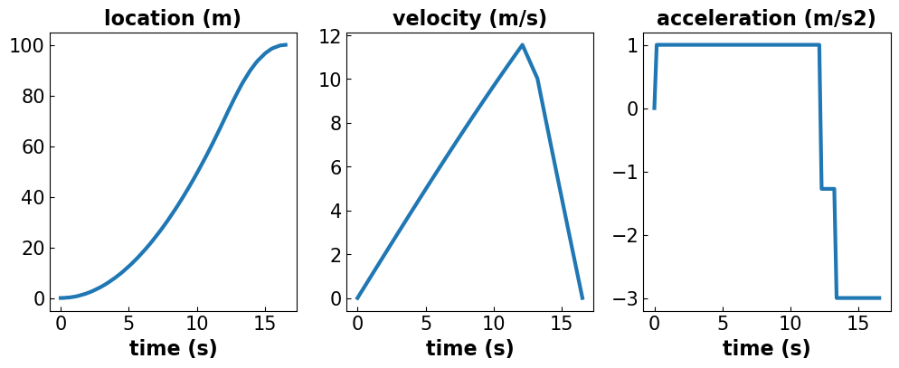
Discussion Questions
How does the time/number of evaluations that IPOPT needs to solve the problem change for a discretized versus non-discretized model?
Why might the two solutions differ?
Check to make sure that these results make sense. Based on the known derivative relationships between position, velocity, and acceleration, do the 3 plots make sense? Hint: Match up the trends in each graph.