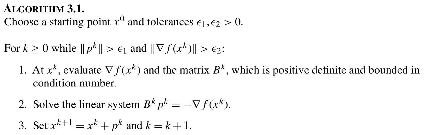
6.5. Quasi-Newton Methods for Unconstrained Optimization#
Reference: Sections 3.1 - 3.3 in Biegler (2010)
# Load required Python libraries.
import matplotlib.pyplot as plt
import numpy as np
from scipy import linalg
6.5.1. Unconstrained Optimization with Approximate Hessian#
SR1 update is one way to approximate \(B^k\).
6.5.1.1. Library of helper functions#
## Check is element of array is NaN
def check_nan(A):
    return np.sum(np.isnan(A))

## Calculate gradient with central finite difference
def my_grad_approx(x,f,eps1,verbose=False):
    '''
    Calculate gradient of function my_f using central difference formula

    Inputs:
        x - point for which to evaluate gradient
        f - function to consider
        eps1 - perturbation size

    Outputs:
        grad - gradient (vector)
    '''

    n = len(x)
    grad = np.zeros(n)

    if(verbose):
        print("***** my_grad_approx at x = ",x,"*****")

    for i in range(0,n):

        # Create vector of zeros except eps in position i
        e = np.zeros(n)
        e[i] = eps1

        # Finite difference formula
        my_f_plus = f(x + e)
        my_f_minus = f(x - e)

        # Diagnostics
        if(verbose):
            print("e[",i,"] = ",e)
            print("f(x + e[",i,"]) = ",my_f_plus)
            print("f(x - e[",i,"]) = ",my_f_minus)


        grad[i] = (my_f_plus - my_f_minus)/(2*eps1)

    if(verbose):
        print("***** Done. ***** \n")

    return grad

## Calculate Hessian using cental finite difference
def my_hes_approx(x,grad,eps2):
    '''
    Calculate gradient of function my_f using central difference formula and my_grad

    Inputs:
        x - point for which to evaluate gradient
        grad - function to calculate the gradient
        eps2 - perturbation size (for Hessian NOT gradient approximation)

    Outputs:
        H - Hessian (matrix)
    '''

    n = len(x)
    H = np.zeros([n,n])

    for i in range(0,n):
        # Create vector of zeros except eps in position i
        e = np.zeros(n)
        e[i] = eps2

        # Evaluate gradient twice
        grad_plus = grad(x + e)
        grad_minus = grad(x - e)

        # Notice we are building the Hessian by column (or row)
        H[:,i] = (grad_plus - grad_minus)/(2*eps2)

    return H

## Linear algebra calculation
def xxT(u):
    '''
    Calculates u*u.T to circumvent limitation with SciPy

    Arguments:
    u - numpy 1D array

    Returns:
    u*u.T

    Assume u is a nx1 vector.
    Recall: NumPy does not distinguish between row or column vectors

    u.dot(u) returns a scalar. This functon returns an nxn matrix.
    '''

    n = len(u)
    A = np.zeros([n,n])
    for i in range(0,n):
        for j in range(0,n):
            A[i,j] = u[i]*u[j]

    return A

## Analyze Hessian
def analyze_hes(B):
    print(B,"\n")

    l = linalg.eigvals(B)
    print("Eigenvalues: ",l,"\n")
6.5.1.2. Symmetric Rank 1 (SR1) Update#
def alg1_sr1(x0,calc_f,calc_grad,eps1,eps2,verbose=False,max_iter=1000):
    '''
    Arguments:
        x0 - starting point
        calc_f - funcation that calculates f(x)
        calc_grad - function that calculates gradient(x)

    Outputs:
        x - iteration history of x (decision variables)
        f - iteration history of f(x) (objective value)
        p - iteration history of p (steps)
        B - Hessian approximation
    '''

    # Allocate outputs as empty lists
    x = []
    f = []
    p = []
    grad = []
    B = []

    # Store starting point
    x.append(x0)
    k = 0

    flag = True

    print("Iter. \tf(x) \t\t||grad(x)|| \t||p|| \t\tmin(lambda)")

    while flag and k < max_iter:
        # Evaluate f(x) at current iteration
        f.append(calc_f(x[k]))

        # Evaluate gradient
        grad.append(calc_grad(x[k]))

        if(check_nan(grad[k])):
            print("WARNING: gradiant calculation returned NaN")
            break

        if verbose:
            print("\n")
            print("k = ",k)
            print("x = ",x[k])
            print("grad = ",grad[k])


        # Update Hessian approximation
        if k == 0:
            # Initialize with identity
            B.append(np.eye(len(x0)))

        else:
            # Change in x
            s = x[k] - x[k-1]

            # Change in gradient
            y = grad[k] - grad[k-1]

            # SR1 formulation
            u = y - B[k-1].dot(s)
            denom = (u).dot(s)

            # Formula: dB = u * u.T / (u.T * s) if u is a column vector.
            dB = xxT(u)/denom

            if(verbose):
                print("s = ",s)
                print("y = ",y)
                print("SR1 update denominator, (y-B[k-1]*s).T*s = ",denom)
                print("SR1 update u = ",u)
                print("SR1 update u.T*u/(u.T*s) = \n",dB)

            B.append(B[k-1] + dB)

        if verbose:
            print("B = \n",B[k])

        if(check_nan(B[k])):
            print("WARNING: Hessian update returned NaN")
            break

        c = np.linalg.cond(B[k])
        if c > 1E12:
            flag = False
            print("Warning: Hessian approximation is near singular.")
            print("B[k] = \n",B[k])

        else:
            # Calculate step
            p.append(linalg.solve(B[k],-grad[k]))

            if verbose:
                print("p = ",p[k])

            # Take step
            x.append(x[k] + p[k])

            # Calculate norms
            norm_p = linalg.norm(p[k])
            norm_g = linalg.norm(grad[k])

            # Calculate eigenvalues of Hessian (for display only)
            ev = np.real(linalg.eigvals(B[k]))

            # print("k = ",k,"\t"f[k],"\t",norm_g,"\t",norm_p)
            print(k,'  \t{0: 1.4e} \t{1:1.4e} \t{2:1.4e} \t{3: 1.4e}'.format(f[k],norm_g,norm_p,np.min(ev)))

            # Check convergence criteria
            flag = (norm_p > eps1) and (norm_g > eps2)

            # Update iteration counter
            k = k + 1

    print("Done.")
    print("x* = ",x[-1])

    return x,f,p,B

print("Done.")
Done.
6.5.2. Test Case: Simple quadratic program#
def my_f_simple(x):
    return x[0]**2 + (x[1]-1)**2

def my_grad_exact(x):
    return np.array([2*x[0], 2*(x[1] - 1) ])
6.5.2.1. Near solution#
Consider \(x_0 = [-0.1, 0.5]^T\)
# Specify convergence criteria
eps1 = 1E-8
eps2 = 1E-4

# Create a Lambda (anonymous) function for gradient calculation
# calc_grad = lambda x : my_grad_approx(x,my_f_simple,1E-6,verbose=False)
calc_grad = lambda x : my_grad_exact(x)

# Specify starting point
x0 = np.array([-0.1, 0.2])

# Call optimization routine
x,f,p,B = alg1_sr1(x0,my_f_simple,calc_grad,eps1,eps2,verbose=False,max_iter=50);

# SR1 Hessian approximation
print("\nSR1 Hessian approximation. B[k] =")
analyze_hes(B[-1])

# Actual Hessian
print("True Hessian at x*. B =")
analyze_hes(my_hes_approx(x[-1],calc_grad,1E-6))
Iter. 	f(x) 		||grad(x)|| 	||p|| 		min(lambda)
0   	 6.5000e-01 	1.6125e+00 	1.6125e+00 	 1.0000e+00
1   	 6.5000e-01 	1.6125e+00 	8.0623e-01 	 1.0000e+00
2   	 1.9259e-34 	2.7756e-17 	2.7595e-17 	 1.0000e+00
Done.
x* =  [1.36642834e-17 1.00000000e+00]

SR1 Hessian approximation. B[k] =
[[1.01538462 0.12307692]
 [0.12307692 1.98461538]]

Eigenvalues:  [1.+0.j 2.+0.j]

True Hessian at x*. B =
[[2. 0.]
 [0. 2.]]

Eigenvalues:  [2.+0.j 2.+0.j]
6.5.2.2. Far from solution#
Consider \(x_0 = [-100, 500]^T\)
# Specify starting point
x0 = np.array([-100, 500])

# Call optimization routine
x,f,p,B = alg1_sr1(x0,my_f_simple,calc_grad,eps1,eps2,verbose=False,max_iter=50);

# SR1 Hessian approximation
print("\nSR1 Hessian approximation. B[k] =")
analyze_hes(B[-1])

# Actual Hessian
print("True Hessian at x*. B =")
analyze_hes(my_hes_approx(x[-1],calc_grad,1E-6))
Iter. 	f(x) 		||grad(x)|| 	||p|| 		min(lambda)
0   	 2.5900e+05 	1.0178e+03 	1.0178e+03 	 1.0000e+00
1   	 2.5900e+05 	1.0178e+03 	5.0892e+02 	 1.0000e+00
2   	 3.4331e-27 	1.1719e-13 	7.2963e-14 	 1.0000e+00
Done.
x* =  [2.46138186e-14 1.00000000e+00]

SR1 Hessian approximation. B[k] =
[[ 1.03860989 -0.19266335]
 [-0.19266335  1.96139011]]

Eigenvalues:  [1.+0.j 2.+0.j]

True Hessian at x*. B =
[[2. 0.]
 [0. 2.]]

Eigenvalues:  [2.+0.j 2.+0.j]
6.5.2.3. Activity/Discussion#
Does the number of iterations depend on the starting point for this problem?
How many iterations are needed for Newton’s method to converge for a positive definite quadratic program using exact second derivative information?
Why does the SR1 update not converge to the true Hessian?
6.5.3. Test Case: Example 2.19#
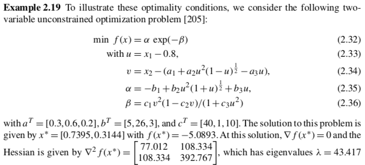
## Define Python function to calculate objective
def my_f_ex_2_19(x,verbose=False):
    ''' Evaluate function given above at point x

    Inputs:
        x - vector with 2 elements

    Outputs:
        f - function value (scalar)
    '''
    # Constants
    a = np.array([0.3, 0.6, 0.2])
    b = np.array([5, 26, 3])
    c = np.array([40, 1, 10])

    # Intermediates. Recall Python indicies start at 0
    u = x[0] - 0.8
    s = np.sqrt(1-u)
    s2 = np.sqrt(1+u)
    v = x[1] -(a[0] + a[1]*u**2*s-a[2]*u)
    alpha = -b[0] + b[1]*u**2*s2+ b[2]*u # September 5, 2018: changed 's' to 's2'
    beta = c[0]*v**2*(1-c[1]*v)/(1+c[2]*u**2)
    f = alpha*np.exp(-beta)

    if verbose:
        print("##### my_f at x = ",x, "#####")
        print("u = ",u)
        print("sqrt(1-u) = ",s)
        print("sqrt(1+u) = ",s2)
        print("v = ",v)
        print("alpha = ",alpha)
        print("beta = ",beta)
        print("f(x) = ",f)
        print("##### Done. #####\n")

    return f
6.5.3.1. \(x_0\) somewhat near solution#
Consider: $\(x_0 = [0.3, 0.1]^T\)$
# Create a Lambda (anonymous) function for gradient calculation
calc_grad = lambda x : my_grad_approx(x,my_f_ex_2_19,1E-6,verbose=False)

# Specify starting point
x0 = np.array([0.3, 0.1])

# Call optimization routine
x,f,p,B = alg1_sr1(x0,my_f_ex_2_19,calc_grad,eps1,eps2,verbose=False,max_iter=250);

# SR1 Hessian approximation
print("\nSR1 Hessian approximation. B[k] =")
analyze_hes(B[-1])

# Actual Hessian
print("True Hessian at x*. B =")
analyze_hes(my_hes_approx(x[-1],calc_grad,1E-6))
Iter. 	f(x) 		||grad(x)|| 	||p|| 		min(lambda)
0   	-3.6022e-02 	8.3847e-01 	8.3847e-01 	 1.0000e+00
1   	-4.1276e-02 	4.7785e-01 	3.0223e-01 	 1.0000e+00
2   	-2.2301e+00 	2.1236e+01 	3.0865e-01 	-6.8856e+01
3   	-4.1260e-02 	4.4645e-01 	1.3053e-01 	-6.7478e+01
4   	-1.0354e-01 	1.1855e+00 	1.5062e-01 	-7.1805e+01
5   	-3.7115e-02 	3.9982e-01 	1.3096e-02 	-5.8783e+01
6   	-3.4039e-02 	3.6164e-01 	5.9865e-02 	-1.4365e+01
7   	-2.2398e-02 	2.0377e-01 	4.2988e-02 	-9.5209e+00
8   	-1.7133e-02 	1.1914e-01 	4.2522e-02 	-6.4394e+00
9   	-1.4292e-02 	5.7282e-02 	2.4810e-02 	-4.8015e+00
10   	-1.3542e-02 	2.5813e-02 	1.0353e-02 	-2.8612e+00
11   	-1.3373e-02 	1.0933e-02 	8.4091e-03 	-1.6117e+00
12   	-1.3325e-02 	7.7765e-04 	7.5906e-04 	-1.6030e+00
13   	-1.3324e-02 	1.7106e-05 	1.4129e-05 	-1.5761e+00
Done.
x* =  [0.80557705 0.96556999]

SR1 Hessian approximation. B[k] =
[[-1.48333926 -0.21589307]
 [-0.21589307 -1.07333656]]

Eigenvalues:  [-1.57605484+0.j -0.98062097+0.j]

True Hessian at x*. B =
[[-1.47002939 -0.20602227]
 [-0.20602227 -1.06561938]]

Eigenvalues:  [-1.55649728+0.j -0.9791515 +0.j]
6.5.3.2. \(x_0\) far from solution#
Consider: $\(x_0 = [-0.1, 0.2]^T\)$
# Specify starting point
x0 = np.array([-0.1, 0.2])

# Call optimization routine
x,f,p,B = alg1_sr1(x0,my_f_ex_2_19,calc_grad,eps1,eps2,verbose=False,max_iter=250);

# SR1 Hessian approximation
print("\nSR1 Hessian approximation. B[k] =")
analyze_hes(B[-1])

# Actual Hessian
print("True Hessian at x*. B =")
analyze_hes(my_hes_approx(x[-1],calc_grad,1E-6))
Iter. 	f(x) 		||grad(x)|| 	||p|| 		min(lambda)
0   	-4.5540e-04 	9.2580e-03 	9.2580e-03 	 1.0000e+00
1   	-5.4879e-04 	1.0959e-02 	5.9578e-02 	-1.8395e-01
2   	-1.5604e-04 	3.4877e-03 	2.7627e-02 	-1.2568e-01
3   	-8.3235e-05 	1.9563e-03 	3.5000e-02 	-5.5390e-02
4   	-3.6006e-05 	9.0023e-04 	2.9559e-02 	-3.0011e-02
5   	-1.7097e-05 	4.4964e-04 	2.9246e-02 	-1.5078e-02
6   	-7.9092e-06 	2.1835e-04 	2.7389e-02 	-7.7836e-03
7   	-3.7242e-06 	1.0745e-04 	2.6349e-02 	-3.9664e-03
8   	-1.7531e-06 	5.2702e-05 	2.5208e-02 	-2.0268e-03
Done.
x* =  [-0.11328951 -0.05033867]

SR1 Hessian approximation. B[k] =
[[ 1.00141633e+00 -4.82365647e-02]
 [-4.82365647e-02  2.91945446e-04]]

Eigenvalues:  [ 1.00373512+0.j -0.00202684+0.j]

True Hessian at x*. B =
[[ 6.99115848e-05 -2.18301460e-04]
 [-2.18301460e-04 -7.02712139e-04]]

Eigenvalues:  [ 0.00012733+0.j -0.00076013+0.j]
6.5.3.3. Activity/Discussion#
Classify each candidate solution.
Is the SR1 approximation always positive definite?
6.5.4. Broyden update with Cholesky factorization#
As part of Algorithms Homework 3, you will adapt this example and implement the BFGS (Broyden-Fletcher-Goldfarb-Shanno) update formula.
You may decide to use the Cholesky factorization of \(B^{k}\),
to make your BFGS update more efficient. (This is not required). Let’s see how to do Cholseky factorization with SciPy.
## Create random P.D. and symmetric matrix
B_ = np.eye(3) + xxT(np.random.normal(0,1,3))
print("B = \n",B_,"\n")

## Perform Cholesky factorization.
# By default, lower=False and L is upper triangular. Either works here,
# but we prefer L to be lower triangular for convention.
L = linalg.cholesky(B_,lower=True)
print("L = \n",L,"\n")

## Reconstruct B
print("L*L.T = \n",L.dot(L.T),"\n")
B =
 [[ 1.00098448  0.00242031 -0.01329946]
 [ 0.00242031  1.00595022 -0.03269612]
 [-0.01329946 -0.03269612  1.17966326]]

L =
 [[ 1.00049212  0.          0.        ]
 [ 0.00241912  1.00296778  0.        ]
 [-0.01329292 -0.03256731  1.08555328]]

L*L.T =
 [[ 1.00098448  0.00242031 -0.01329946]
 [ 0.00242031  1.00595022 -0.03269612]
 [-0.01329946 -0.03269612  1.17966326]]