3.2. Numeric Integration for DAEs#

Prepared by: Prof. Alexander Dowling, Myia Dickens (mdicken2@nd.edu,2023)

The purpose of this notebook/class session is to provide the requisite background on numeric integration of DAEs. This helps appreciate the “direct transcription” approach for dynamic optimization used in Pyomo.dae.

import numpy as np
import scipy.optimize as opt
import matplotlib.pyplot as plt

3.2.1. Single-Step Runge-Kutta Methods#

Chapter 9 in Biegler (2010)
Chapter 17 in McClarren (2018)

3.2.1.1. General Form: Index 0 DAE#

Consider the ODE system: $$\begin{equation*} \dot{z} = f(t,z), \quad z(t_0) = z_0 \end{equation*}$$

where $z(t)$ are the differentail variables and $f(t,z)$ is a (nonlinear) continous function.

The general Runge-Kutta formula is: $$\begin{align*} z_{i+1} &= z_{i} + h_i \sum_{k=1}^{n_s} b_k f(t_i + c_k h_i, \hat{z}_k) \\ \hat{z}_k &= z_i + h_i \sum_{j=1}^{n_{rk}} a_{k,j} f(t_i + c_j h_i, \hat{z}_j), \quad k=1,...,n_s \end{align*}$$

where

$z_i$ are the differential variables at the start of step $i$ (time $t_i$)
$z_{i+1}$ are the differential variables at the end of step $i$ (time $t_{i+1}$)
$\hat{z}_k$ are differential variables for intermediate stage $k$
$h_i$ is the size for step $i$ such that $t_{i+1} = t_i + h_i$
$n_s$ is the number of stages
$n_{rk}$ is the number of $f(\cdot)$ evaluations to calculate intermediate $k$
$a_{k,j}$ are coefficients, together known as the Runge-Kutta matrix
$b_k$ are cofficients, known as the weights
$c_k$ are coefficients, know as the nodes

$h_i$ is selected based on error tolerances

The choice for $A$, $b$ and $c$ selects the specific method in the Runge-Kutta family. These coefficients are often specific in a Butcher block (or Butcher tableau).

A Runge-Kutta method is called consistent if: $$\begin{equation*} \sum_{k=1}^{n_s} b_k = 1 \quad \mathrm{and} \quad \sum_{j=1}^{n_s} a_{k,j} = c_k \end{equation*}$$

3.2.1.2. Explicit (Forward) Euler#

Consider one of the simplest Runge-Kutta methods:

\[z_{i+1} = z_{i} + h_i~f(t_i, z_i)\]

What are $A$, $b$ and $c$ in the general formula?

$n_s = 1$. This is only a single stage. Thus we only need to determine $c_1$, $b_1$, and $n_{r1}$

Moreover, $\hat{z}_1 = z_i$ because $f(\cdot)$ is only evaluated at $t_i$ and $z_i$. This implies:

$n_{r1} = 0$
$c_1 = 0$
$b_1 = 1$
$A$ is empty because $n_{r1} = 0$

The implementation is very straightword (see below). We can calculate $z_{i+1}$ with a single line!

def create_steps(tstart,tend,dt):
    n = int(np.ceil((tend-tstart)/dt))
    return dt*np.ones(n)

def explicit_euler(f,h,z0):
    '''
    Arguments:
        f: function that returns rhs of ODE
        h: list of step sizes
        z0: initial conditions
        
    Returns:
        t: list of time steps. t[0] is 0.0 by default
        z: list of differential variable values
    '''
    
    # Number of timesteps
    nT = len(h) + 1
    
    t = np.zeros(nT)
    
    # Number of states
    nZ = len(z0)
    Z = np.zeros((nT,nZ))
    
    # Copy initial states
    Z[0,:] = z0
    
    for i in range(1,nT):
        
        i_ = i-1
        
        # Advance time
        t[i] = t[i_] + h[i_]
        
        # Implicit Euler formula
        Z[i,:] = Z[i_,:] + h[i_]*f(t[i_],Z[i_,:])
        
    return t, Z

3.2.1.3. Implicit (Backward) Euler#

Consider another simple Runge-Kutta method:

\[z_{i+1} = z_{i} + h_i~f(t_{i+1}, z_{i+1})\]

What are $A$, $b$ and $c$ to express using the general formula?

$n_s = 1$. Thus is only a single stage. Moreover, $\hat{z}_1 = z_{i+1}$ because $f(\cdot)$ is evaluated at $t_{i+1}$ and $z_{i+1}$. This implies:

$b_1 = 1$
$c_1 = 1$

Moreover, $z_{i+1} = z_{i} + h_i~f(t_{i+1}, z_{i+1})$ implies $\hat{z}_1 = z_i + h_i f(t_{i+1}, \hat{z}_1)$. Thus:

$a_{1,1} = 1$

Notice that the formula for $z_{i+1}$ is implicit. We need to solve a (nonlinear) system of equations to calculate the step.

def implicit_euler(f,h,z0):
    '''
    Arguments:
        f: function that returns rhs of ODE
        h: list of step sizes
        z0: initial conditions
        
    Returns:
        t: list of time steps. t[0] is 0.0 by default
        z: list of differential variable values
    '''
    
    # Number of timesteps
    nT = len(h) + 1
    
    t = np.zeros(nT)
    
    # Number of states
    nZ = len(z0)
    Z = np.zeros((nT,nZ))
    
    # Copy initial states
    Z[0,:] = z0
    
    for i in range(1,nT):
        
        i_ = i-1
        
        # Advance time
        t[i] = t[i_] + h[i_]
        
        ## Implicit Runge-Kutta formula.
        ## Need to solve nonlinear system of equations.
        
        # Use Explicit Euler to calculate initial guess
        Z[i,:] = Z[i_,:] + h[i_]*f(t[i_],Z[i_,:])
        
        # Solve nonlinear equation
        implicit = lambda z : Z[i_,:] + h[i_]*f(t[i_],z) - z
        Z[i,:] = opt.fsolve(implicit, Z[i,:])
        
        
    return t, Z

3.2.2. Key Differences#

Explicit Methods	Implicit Methods
+ Easy to Program	+ Requires converging system of nonlinear equations
- $h_i$ is limited by Stability	+ Stability is independent of $h_i$

3.2.2.1. Comparison#

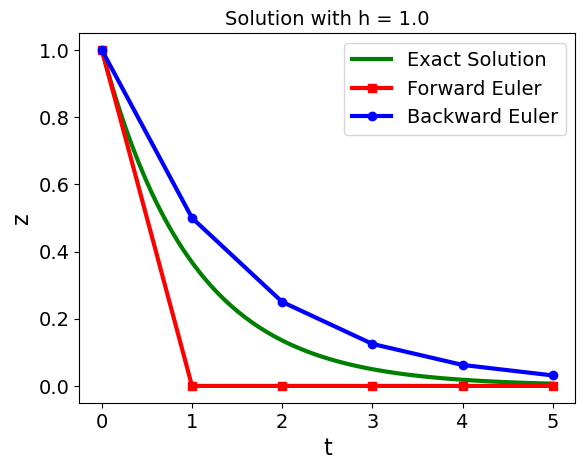
Let’s test this on a simple problem: $$\dot{z}(t) = -\lambda z(t), \qquad z_0 = 1.$$ The solution to this problem is $$z(t) = e^{-\lambda t}.$$

For simplicity, let’s numerically analyze $\lambda = 1$.

rhs = lambda t, z: -z
sln = lambda t: np.exp(-t)

dt = 1.0
h = create_steps(0.0,5.0,dt)

z0 = [1]

te, Ze = explicit_euler(rhs, h, z0)
ti, Zi = implicit_euler(rhs, h, z0)

plt.figure()

# Use 101 points for exact to make it smooth
texact = np.linspace(0.0,np.sum(h),101)

# Plot solutions
plt.plot(texact, sln(texact),color='green',label="Exact Solution")
plt.plot(te,Ze,color='red',marker='s',label='Forward Euler')
plt.plot(ti,Zi,color='blue',marker='o',label='Backward Euler')
plt.xlabel('t')
plt.ylabel('z')
plt.legend()
plt.title('Solution with h = '+ str(dt))
plt.show()

../../_images/DAE_numeric_integration_10_0.png

3.2.2.2. Stability#

Keeping $\lambda = 1$, are there any limits on step size?

dt = 2.5
h = create_steps(0.0,10.0,dt)

z0 = [1]

te, Ze = explicit_euler(rhs, h, z0)
ti, Zi = implicit_euler(rhs, h, z0)

plt.figure()

# Use 101 points for exact to make it smooth
texact = np.linspace(0.0,np.sum(h),101)

# Plot solutions
plt.plot(texact, sln(texact),color='green',label="Exact Solution")
plt.plot(te,Ze,color='red',marker='s',label='Forward Euler')
plt.plot(ti,Zi,color='blue',marker='o',label='Backward Euler')
plt.xlabel('t')
plt.ylabel('z')
plt.legend()
plt.title('Solution with h = '+ str(dt))
plt.show()

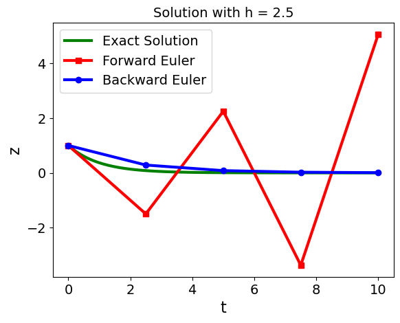
../../_images/DAE_numeric_integration_12_0.png

Key observation: forward (explicit) Euler becomes unstable with large steps whereas backward (implicit) Euler is stable.

There is a good mathematical reason for this! See http://www.it.uu.se/edu/course/homepage/bridging/ht13/Stability_Analysis.pdf for details.

Key results (for this specific test problem):

Explicit Euler requires step sizes with $h < 2/\lambda$.
Implicit Euler is unconditionally stable provided $\lambda > 0$.
Similar analysis and concepts extend to Runge-Kutta methods.

3.2.2.3. Error Analysis#

How does our choice in step size $h$ impact the error of these numerical techniques?

Delta_t = np.array([1.0,.5,.25,.125,.0625,.0625/2])
t_final = 2
error_forward = np.zeros(Delta_t.size)
error_backward = np.zeros(Delta_t.size)

for i in range(0,len(Delta_t)):
    
    # create steps
    h = create_steps(0.0,t_final,Delta_t[i])
    
    # solve
    t,ze = explicit_euler(rhs, h, z0)
    t,zi = implicit_euler(rhs, h, z0)
    zsln = np.exp(-t)
    
    n = len(t) - 1
    
    # Calculate error
    error_forward[i] = np.linalg.norm(ze[:,0] - zsln)/np.sqrt(n)
    error_backward[i] = np.linalg.norm(zi[:,0] - zsln)/np.sqrt(n)
    

plt.loglog(Delta_t,error_forward,'s-',color="red",label="Forward Euler")
plt.loglog(Delta_t,error_backward,'o-',color="blue",label="Backward Euler")

#slope = (np.log(error[-1]) - np.log(error[-2]))/(np.log(Delta_t[-1])- np.log(Delta_t[-2]))
#plt.title("Slope of Error is " + str(slope))
plt.xlabel("Step Size (h)")
plt.ylabel("Norm of Error")
plt.show()

# Calculate slope
calc_slope = lambda error: (np.log(error[-1]) - np.log(error[-2]))/(np.log(Delta_t[-1])- np.log(Delta_t[-2]))

print("Slope for Forward Euler: " + str(calc_slope(error_forward)))
print("Slope for Backward Euler: " + str(calc_slope(error_backward)))

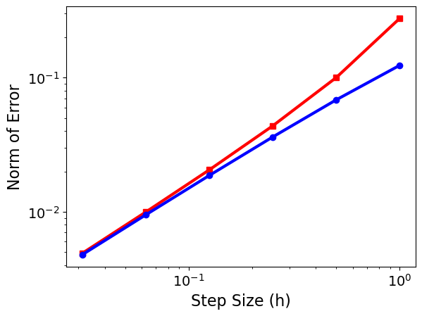
../../_images/DAE_numeric_integration_15_0.png

Slope for Forward Euler: 1.0220608473216777
Slope for Backward Euler: 0.9874086317220228

Notice that the error indicates that this is a first-order method in $\Delta t$: when I decrease $\Delta t$ by a factor of 2, the error decreases by a factor of 2. In this case we measured the error with a slightly different error norm: $$\mathrm{Error} = \frac{1}{\sqrt{N}}\sqrt{\sum_{n=1}^{N} \left(y^n_\mathrm{approx} - y^n_\mathrm{exact}\right)^2},$$ where $N$ is the number of steps the ODE is solved over.

Key Results:

Implicit and Explicit Euler have $O(h^2)$ local error and $O(h)$ global error.

3.2.3. Extending Numeric Integration to Index-1 DAEs#

Consider semi-explicit DAEs: $$\begin{equation*} \dot{z} = f(t,z,y), \quad g(z,y) = 0, \quad z(t_0) = z_0 \end{equation*}$$

Runge-Kutta methods are easy to extend.

\[\begin{split}\begin{align*} z_{i+1} &= z_{i} + h_i \sum_{k=1}^{n_s} b_k f(t_i + c_k h_i, \hat{z}_k, \hat{y}_k) \\ \hat{z}_k &= z_i + h_i \sum_{j=1}^{n_{rk}} a_{k,j} f(t_i + c_j h_i, \hat{z}_j, \hat{y}_j), \quad k=1,...,n_s \\ 0 &= g(\hat{z}_k, \hat{y}_k), \quad k=1,...,n_s \end{align*}\end{split}\]

The Backwards Euler is also another method to use to extend.

\[\begin{split}\begin{align*} z_{i+1} &= \sum_{j=1}^{n_s} \alpha_j z_{i-j+1} + \beta_0 hf(z_{i+1},y_{i+1})\\ 0 &= g(z_{i+1},y_{i+1}) \end{align*}\end{split}\]

If using the Backwards Euler, the solution can be found using Newton’s method and the Jacobian given by:

\[\begin{split}\begin{align*} J(z_{i+1},y_{i+1}) &= \begin{bmatrix} I - h\beta_0\frac{\partial f}{\partial z}^T & h\beta_0\frac{\partial f}{\partial z}^T \\ \frac{\partial g}{\partial z}^T & \frac{\partial g}{\partial y}^T \end{bmatrix} \end{align*}\end{split}\]

Key Results. If DAE is index 1, then similar stability and order properties as for ODE problems.

Discussion: Why are implicit RK methods always used for DAE systems?

3.2.3.1. Solving Index-1 DAEs using Backwards Euler Method#

Reference: Pyomo - Optimization Modeling in Python (Hart, 2010)

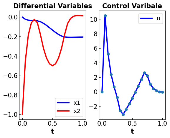
Consider the following optimal control problem

\[\begin{split} $$\begin{align*} \min \quad & x_3(t_f) \\ \mathrm{s.t.} \quad & \dot{x}_1 = x_2 \\ & \dot{x}_2 = -x_2 + u \\ & \dot{x}_3 = x_1^2 + x_2^2 + 0.005 \cdot u^2 \\ & x_2 - 8 \cdot((t-0.5)^2+0.5 \leq 0 \\ & x_1(0) = 0, x_2(0) = 01, x_3(0) = 0, t_f = 1 \end{align*} \end{split}\]

Discussion: What variable is the problem attempting to minimize? What variable is being optimized? What are the types of equations are there?

### Begin Solution
Minimizing variable: u
Optimized varibale: x3
Types of equations: 3 differential equations in the constraints and a path constraint, which is an inequality constraint restricting a varibale. 
In this case, the variable being constricted in x2.

### End Solution

import sys
if "google.colab" in sys.modules:
    !wget "https://raw.githubusercontent.com/ndcbe/CBE60499/main/notebooks/helper.py"
    import helper
    !pip install casadi
    helper.install_idaes()
    helper.install_ipopt()
    helper.install_glpk()
else:
    import idaes # loads Ipopt with HSL

--2023-04-23 15:15:40--  https://raw.githubusercontent.com/ndcbe/CBE60499/main/notebooks/helper.py
Resolving raw.githubusercontent.com (raw.githubusercontent.com)... 185.199.108.133, 185.199.109.133, 185.199.110.133, ...
Connecting to raw.githubusercontent.com (raw.githubusercontent.com)|185.199.108.133|:443... connected.
HTTP request sent, awaiting response... 200 OK
Length: 7171 (7.0K) [text/plain]
Saving to: ‘helper.py.1’


helper.py.1           0%[                    ]       0  --.-KB/s               
helper.py.1         100%[===================>]   7.00K  --.-KB/s    in 0s      

2023-04-23 15:15:40 (92.0 MB/s) - ‘helper.py.1’ saved [7171/7171]

Looking in indexes: https://pypi.org/simple, https://us-python.pkg.dev/colab-wheels/public/simple/
Requirement already satisfied: casadi in /usr/local/lib/python3.9/dist-packages (3.6.1)
Requirement already satisfied: numpy in /usr/local/lib/python3.9/dist-packages (from casadi) (1.22.4)
IDAES found! No need to install.
Running idaes get-extensions to install Ipopt, k_aug, and more...
Ipopt 3.13.2 (x86_64-pc-linux-gnu), ASL(20190605)

[K_AUG] 0.1.0, Part of the IDAES PSE framework
Please visit https://idaes.org/ (x86_64-pc-linux-gnu), ASL(20190605)

Couenne 0.5.8 -- an Open-Source solver for Mixed Integer Nonlinear Optimization
Mailing list: couenne@list.coin-or.org
Instructions: http://www.coin-or.org/Couenne
couenne (x86_64-pc-linux-gnu), ASL(20190605)

Bonmin 1.8.8 using Cbc 2.10.8 and Ipopt 3.13.2
bonmin (x86_64-pc-linux-gnu), ASL(20190605)

Ipopt 3.13.3 (x86_64-pc-linux-gnu), ASL(20190605)

ipopt was successfully installed
k_aug was successfuly installed
cbc was successfuly installed
clp was successfuly installed
bonmin was successfuly installed
couenne was successfuly installed
ipopt_l1 was successfuly installed
 
Installing glpk via apt-get...

import pyomo.environ as pyo
import pyomo.dae as dae

def create_model_index1():

  # Create model
  m = pyo.ConcreteModel()

  # Declare time set
  m.tf = pyo.Param(initialize = 1) #final time
  m.t = dae.ContinuousSet(bounds=(0,m.tf))

  # Declare constraint and input variables
  m.u = pyo.Var(m.t, initialize = 0)
  m.x1 = pyo.Var(m.t)
  m.x2 = pyo.Var(m.t)
  m.x3 = pyo.Var(m.t)

  # Declare differential variables
  m.dx1 = dae.DerivativeVar(m.x1, wrt=m.t)
  m.dx2 = dae.DerivativeVar(m.x2, wrt=m.t)
  m.dx3 = dae.DerivativeVar(m.x3)

  # Declare differential equations
  def _x1dot(m,t):
    if t == m.t.first():
      return pyo.Constraint.Skip
    return m.dx1[t] == m.x2[t]
  m.x1dotcon = pyo.Constraint(m.t, rule=_x1dot)

  def _x2dot(m,t):
    if t == m.t.first():
      return pyo.Constraint.Skip
    return m.dx2[t] == -m.x2[t] + m.u[t]
  m.x2dotcon = pyo.Constraint(m.t, rule=_x2dot)

  def _x3dot(m,t):
    if t == m.t.first():
      return pyo.Constraint.Skip
    return m.dx3[t] == m.x1[t]**2+m.x2[t]**2+0.005*m.u[t]**2
  m.x3dotcon = pyo.Constraint(m.t, rule=_x3dot)

  # Declare inequality constraints
  def _con(m,t):
    return m.x2[t]-8*(t-0.5)**2+0.5 <= 0
  m.con = pyo.Constraint(m.t, rule = _con)

  # Declare the intial conditions
  def _init(m):
    yield m.x1[0] == 0
    yield m.x2[0] == -1
    yield m.x3[0] == 0
  m.init_conditions = pyo.ConstraintList(rule=_init)

  # Declare Objective function
  m.obj = pyo.Objective(expr = m.x3[m.tf])

  return m

# Solve model using Backwards Euler Method
def dae_index1_BackEuler(m):
  '''
    Arguments:
      m: DAE model of Index 1
    New Elements:
      nfe = number for finite elements - specifies the number of discretization points to be used
    Purpose:
      Solves DAE model using Backwards Euler method
  '''

  discretizer = pyo.TransformationFactory('dae.finite_difference')
  discretizer.apply_to(m, nfe=20, wrt=m.t, scheme = 'BACKWARD')

  solver = pyo.SolverFactory('ipopt')
  results = solver.solve(m, tee = True)

# Plot the results
def plotter(subplot, x, *y, **kwds):
  plt.subplot(subplot)
  for i,_y in enumerate(y):
    plt.plot(list(x), [pyo.value(_y[t]) for t in x], 'brgcmk' [i%6])
    if kwds.get('points',False):
      plt.plot(list(x), [pyo.value(_y[t]) for t in x], 'o')
  plt.title(kwds.get('title',''),fontsize = 16, fontweight='bold')
  plt.tick_params(direction="in",labelsize=15)
  plt.legend(tuple(_y.name for _y in y))
  plt.xlabel(x.name, fontsize = 16, fontweight='bold')


def plot_results(m):
  plotter(121, m.t, m.x1, m.x2, title = 'Differential Variables')
  plotter(122, m.t, m.u, title='Control Varibale', points=True)
  plt.show()

# Create model
model = create_model_index1()

# Solve DAEs
results = dae_index1_BackEuler(model)

Ipopt 3.13.2: 

******************************************************************************
This program contains Ipopt, a library for large-scale nonlinear optimization.
 Ipopt is released as open source code under the Eclipse Public License (EPL).
         For more information visit http://projects.coin-or.org/Ipopt

This version of Ipopt was compiled from source code available at
    https://github.com/IDAES/Ipopt as part of the Institute for the Design of
    Advanced Energy Systems Process Systems Engineering Framework (IDAES PSE
    Framework) Copyright (c) 2018-2019. See https://github.com/IDAES/idaes-pse.

This version of Ipopt was compiled using HSL, a collection of Fortran codes
    for large-scale scientific computation.  All technical papers, sales and
    publicity material resulting from use of the HSL codes within IPOPT must
    contain the following acknowledgement:
        HSL, a collection of Fortran codes for large-scale scientific
        computation. See http://www.hsl.rl.ac.uk.
******************************************************************************

This is Ipopt version 3.13.2, running with linear solver ma27.

Number of nonzeros in equality constraint Jacobian...:      363
Number of nonzeros in inequality constraint Jacobian.:       21
Number of nonzeros in Lagrangian Hessian.............:       60

Total number of variables............................:      143
                     variables with only lower bounds:        0
                variables with lower and upper bounds:        0
                     variables with only upper bounds:        0
Total number of equality constraints.................:      123
Total number of inequality constraints...............:       21
        inequality constraints with only lower bounds:        0
   inequality constraints with lower and upper bounds:        0
        inequality constraints with only upper bounds:       21

iter    objective    inf_pr   inf_du lg(mu)  ||d||  lg(rg) alpha_du alpha_pr  ls
   0  0.0000000e+00 1.00e+00 2.82e-01  -1.0 0.00e+00    -  0.00e+00 0.00e+00   0
   1  0.0000000e+00 1.24e+00 6.10e-01  -1.0 1.57e+01    -  6.19e-01 1.00e+00f  1
   2  3.3913637e-01 2.47e-01 1.00e-06  -1.0 5.83e+00    -  1.00e+00 1.00e+00f  1
   3  3.3096072e-01 1.37e-02 2.00e-07  -1.7 1.05e+00    -  1.00e+00 1.00e+00h  1
   4  1.5256107e-01 5.24e-02 1.50e-09  -3.8 9.83e-01    -  1.00e+00 1.00e+00h  1
   5  1.4973078e-01 9.43e-03 1.50e-09  -3.8 6.08e-01    -  1.00e+00 1.00e+00h  1
   6  1.4923815e-01 1.41e-03 1.50e-09  -3.8 3.46e-01    -  1.00e+00 1.00e+00h  1
   7  1.4795692e-01 3.28e-04 4.99e-05  -5.7 1.84e-01    -  1.00e+00 9.88e-01h  1
   8  1.4798373e-01 1.22e-05 1.84e-11  -5.7 3.85e-02    -  1.00e+00 1.00e+00h  1
   9  1.4796950e-01 7.16e-08 2.51e-14  -8.6 2.69e-03    -  1.00e+00 1.00e+00h  1
iter    objective    inf_pr   inf_du lg(mu)  ||d||  lg(rg) alpha_du alpha_pr  ls
  10  1.4796952e-01 6.90e-13 2.51e-14  -8.6 1.15e-05    -  1.00e+00 1.00e+00h  1

Number of Iterations....: 10

                                   (scaled)                 (unscaled)
Objective...............:   1.4796951825372689e-01    1.4796951825372689e-01
Dual infeasibility......:   2.5063284780912909e-14    2.5063284780912909e-14
Constraint violation....:   6.9011463210699731e-13    6.9011463210699731e-13
Complementarity.........:   2.5060342008003915e-09    2.5060342008003915e-09
Overall NLP error.......:   2.5060342008003915e-09    2.5060342008003915e-09


Number of objective function evaluations             = 11
Number of objective gradient evaluations             = 11
Number of equality constraint evaluations            = 11
Number of inequality constraint evaluations          = 11
Number of equality constraint Jacobian evaluations   = 11
Number of inequality constraint Jacobian evaluations = 11
Number of Lagrangian Hessian evaluations             = 10
Total CPU secs in IPOPT (w/o function evaluations)   =      0.010
Total CPU secs in NLP function evaluations           =      0.000

EXIT: Optimal Solution Found.


# Plot solution
plot_results(model)

../../_images/DAE_numeric_integration_25_0.png

Nonlinear and Stochastic Optimization

Numeric Integration for DAEs

Contents