Homework 2: Optimization

Homework 2: Optimization#

Your Name:

Homework assigment 2 is intended to develop your skills in creating linear programming models. The lecture notes will provide with a starting point for the following exercises. The problem data has been changed to provide a more meaningful example for sensitivity analysis.

Blending and Metal Recycling#

You have been placed in charge of a metals reuse operation. A collection of raw materials are available with key parameters given in the following table.

material	% carbon (C)	% copper (Cu)	% manganese (Mn)	amount (kg)	cost ($/kg)	type
1	2.5	0.0	1.3	4000	1.20	iron alloy
2	3.0	0.0	0.8	3000	1.50	iron alloy
3	0.0	0.3	0.0	6000	0.90	iron alloy
4	0.0	90.0	0.0	5000	1.30	copper alloy
5	0.0	96.0	4.0	2000	1.45	copper alloy
6	0.0	0.4	1.2	3000	1.20	aluminum alloy
7	0.0	0.6	0.0	2500	1.00	aluminum alloy

A customer has requested 5000 kg of mix satisfying these specifications:

Component	min %	max %
C	2.0	3.0
Cu	0.4	0.6
Mn	1.2	1.65

You want to develop a Python program to explore the lower cost strategy to fullfill this and similar customer orders.

For convenience, the raw material data has been organized as a nested dictionaries and stored in a pandas DataFrame.

import sys
if "google.colab" in sys.modules:
    !wget "https://raw.githubusercontent.com/IDAES/idaes-pse/main/scripts/colab_helper.py"
    import colab_helper
    colab_helper.install_idaes()
    colab_helper.install_ipopt()

import pandas as pd

materials_data = pd.DataFrame.from_dict({
    "1": {"C": 2.5, "Cu": 0.0, "Mn": 1.3, "amount": 4000, "cost": 1.20},
    "2": {"C": 3.0, "Cu": 0.0, "Mn": 0.8, "amount": 3000, "cost": 1.50},
    "3": {"C": 0.0, "Cu": 0.3, "Mn": 0.0, "amount": 6000, "cost": 0.90},
    "4": {"C": 0.0, "Cu": 90.0, "Mn": 0.0, "amount": 5000, "cost": 1.30},
    "5": {"C": 0.0, "Cu": 96.0, "Mn": 4.0, "amount": 2000, "cost": 1.45},
    "6": {"C": 0.0, "Cu": 0.4, "Mn": 1.2, "amount": 3000, "cost": 1.20},
    "7": {"C": 0.0, "Cu": 0.6, "Mn": 0.0, "amount": 2500, "cost": 1.00},
}).T

display(materials_data)

The product specifications are also available in a pandas DataFrame.

product_composition_specs = pd.DataFrame.from_dict({
    "min": {"C": 2.0, "Cu": 0.4, "Mn": 1.2},
    "max": {"C": 3.0, "Cu": 0.6, "Mn": 1.65}
})

display(product_composition_specs)

Exercise 1. Mathematical Modeling#

On paper, develop a mathematical model for this problem. Similar to class, identify and describe the notation (with units) for sets, variables, and parameters/data. Then write the optimization problem with the mathematical formulation on the left. On the right, add a few words to describe each objective, constraint, and bound. (This is the same format as the examples we did in class.) Please turn in the complete annotated model.

Exercise 2. Pyomo Implementation#

Complete the function below. Follow the style of the class examples on linear blending (beer, gasoline). Hint: Add one constraint at a time.

import pyomo.environ as pyo

def calculate_cost(materials_data, product_composition_specs, batch_size=5000, verbose=False, surpress_output=False):
    ''' Calculate minimum cost of metal blending

    Arguments:
        materials_data: pandas DataFrame
        product_composition_specs: pandas DataFrame
        batch_size: float
        verbose: bool

    Returns:
        solution: dict with the following keys [units]
            - batch [kg of product]
            - A, B, C, D, E, F, G [kg of raw material] 
            - C, Cu, Mn [wt% of final product]
            - cost [$]
            - cost_per_unit [$/kg of product] 

    '''


    m = pyo.ConcreteModel("Metal Blending")

    m.MATERIALS = pyo.Set(initialize=materials_data.index)
    m.ELEMENTS = pyo.Set(initialize=materials_data.columns[:-2])

    m.x = pyo.Var(m.MATERIALS, domain=pyo.NonNegativeReals)

    @m.Objective(sense=pyo.minimize)
    def cost(m):
        return sum(m.x[i]*materials_data.loc[i, "cost"] for i in m.MATERIALS)
    
    
    @m.Constraint(m.ELEMENTS)
    def min_element(m, e):
        return sum(m.x[i]*(materials_data.loc[i, e] - product_composition_specs.loc[e,"max"]) for i in m.MATERIALS) <= 0
    
        
    '''You need to add the constraints here.

    This code will run but give you the wrong answer if
    you don't add the constraints.
    '''
    # Add your solution here

    # solver = pyo.SolverFactory('gurobi')
    solver = pyo.SolverFactory('cbc')

    results = solver.solve(m,tee=verbose)

    if verbose:
        m.pprint()

    solution = {}

    # Amount of each material used
    for i in m.MATERIALS:
        solution[i] = pyo.value(m.x[i])

    # Total amount
    solution['batch'] = sum(solution[i] for i in m.MATERIALS)

    # Composition of the final product
    for e in m.ELEMENTS:
        solution[e] = sum(materials_data.loc[i, e]*solution[i] for i in m.MATERIALS)/solution['batch']

    # Cost
    solution['cost'] = m.cost()

    # Cost per unit
    solution['cost_per_unit'] = solution['cost']/solution['batch']

    solution['status'] = results.solver.status

    if not surpress_output:
        display(pd.DataFrame.from_dict(solution, orient='index', columns=['Value']))
    
    return solution
    
sln = calculate_cost(materials_data, product_composition_specs, batch_size=5000, verbose=False)

What is the minimum price you would need to charge in $/kg to produce 5,000 kg of requested product?

Answer:

Exercise 3. Sensitivity Analysis#

One of the important reasons to create optimization models is to understand the value of the raw materials that are available to you, and how to adjust operations to accomodate changing requirements. The is commonly referred to as sensitivity analysis.

Using the functions you’ve created in above exercises, answer the following questions:

Question 1. The customer is very pleased with your initial pricing for 5,000 kg of the desired product, and now wishes to increase the order to 6,000 kg. Does your unit cost ($/kg) go up? If so, explain why your unit cost has gone up.

# Add your solution here

Answer:

Question 2. Is there an upper limit on how much product your can provide to this customer? (Use trial and error. To the nearest 100 kg, find the maximum amount of product you can ship to the customer.) What is the unit cost now?

# Add your solution here

Answer:

Question 3. After some negotiation, you and your customer settle on an order of 6,500 kg. Now you wish to negotiate with your suppliers for more raw material. How much money do you save for 1 additional kg of raw material “1”? Based on this, what price would you be willing to pay your supplier for additional “A”?

# Add your solution here

Answer:

Data-Driven Portfolio Optimization#

Portfolio management is a classic example of quadratic programming (optimization). The idea is to find the optimal blend of investments that achieves a specified rate of return (or better) while minimizing the variance in rate of return. In this problem, you will use your skills in statistical analysis to analyze the stock data.

Historical Stock Data#

Historical daily adjusted closing prices for the last five years (obtained from Yahoo! Finance) are available for the $N=5$ stocks listed in table below. (We are actually considering index funds, but this detail does not change the analysis.)

Symbol	Name
GSPC	S&P 500
DJI	Dow Jones Industrial Average
IXIC	NASDAQ Composite
RUT	Russell 2000
VIX	CBOE Volatility Index

Return Rate#

You are given a Stock_Data.csv file. Using the stock data, calculate the 1-day return rate:

(6)#\[\begin{equation} r_{t,i} = \frac{p_{t+1,i} - p_{t,i}}{p_{t,i}} \end{equation}\]

where $p_{t+1,i}$ and $p_{t,i}$ are the Adjusted Closing Prices at the end of days $t+1$ and $t$, respectively, for stock $i$. These results are stored in matrix R. Hint: Use Pandas.

# This is the long path to the folder containg data files on GitHub (for the class website)
data_folder = 'https://raw.githubusercontent.com/ndcbe/data-and-computing/main/notebooks/data/'

# Load the data file into Pandas
df_adj_close = pd.read_csv(data_folder + 'Stock_Data.csv')

# Define an empty list to store the return rates
R = []

# Loop over the days (rows) in the data frame
for i in range(len(df_adj_close)):

    # Compute the return rate and append it to the list R
    if i >0:
        # Skip calculation for the first row (day 0)
        R.append((df_adj_close.iloc[i] - df_adj_close.iloc[i-1])/(df_adj_close.iloc[i-1]))

# Convert the list R to a data frame
R = pd.DataFrame(R)

# Print the first 5 return rates
print("\nFirst 5 Return Rates:")
R.head()

Exercise 1. Visualization#

Plot the single day return rates for the 5 stocks you obtain in the previous section and check if you obtain the following profiles:

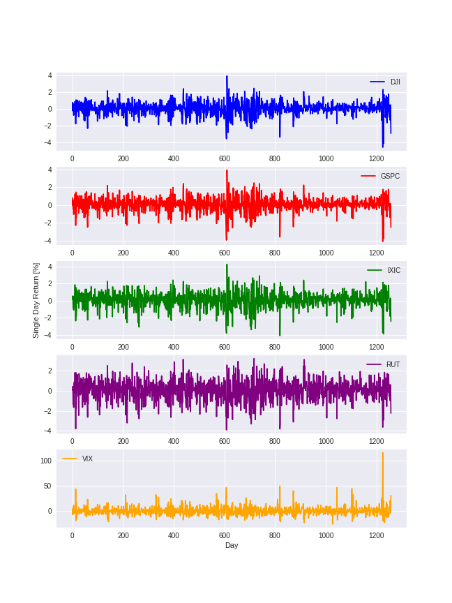
The first plot is made for you.

# Create figure
import matplotlib.pyplot as plt
plt.figure(figsize=(9,15))

# Create subplot for DJI
plt.subplot(5,1,1)
plt.plot(R["DJI"]*100,color="blue",label="DJI")
plt.legend(loc='best')

# Add your solution here

# Show plot
plt.show()

Exercise 2. Covariance and Correlation Matrices#

Write Python code to:

Calculate $\bar{r}$, the average 1-day return for each stock. Store this as the variable R_avg.
Calculate $\Sigma_{r}$, the covariance matrix of the 1-day returns. This matrix tells us how returns for each stock vary with each other (which is important because they are correlated!). Hint: pandas has a function cov
Calculate the correlation matrix for the 1-day returns. Hint: pandas has a function corr.

Looking at the correlation matrix, answer the follwing questions:

Which pair of stocks have the highest positive correlation?
Which pair of stocks have the highest negative correlation?
Which pair of stocks have the lowest absolute correlation?

Hint: Review the CBE 20258 class website for more information on correlation and covariance

Please write one or two sentences for each of the above questions:

Fill in here
Fill in here
Fill in here

# Add your solution here

Exercise 3. Markowitz Mean/Variance Portfolio Optimization Model#

The Markowitz mean/variance model, shown below, computes the optimal allocation of funds in a portfolio:

(7)#\[\begin{align} \min_{{x} \geq {0}} \qquad & z:= {x}^T \cdot {\Sigma_r} \cdot {x} \\ \text{s.t.} \qquad & {\bar{r}}^T \cdot {x} \geq \rho \\ & \sum_{i =1}^N x_i = 1 \end{align}\]

where $x_i$ is the fraction of funds invested in stock $i$ and $x = [x_1, x_2, ..., x_N]^T$. The objective is to minimize the variance of the return rate. (As practice for the next exam, try deriving this from the error propagation formulas.) This requires the expected return rate to be at least $\rho$. Finally, the allocation of funds must sum to 100%.

Write Python code to solve for $\rho = 0.08\%.$ Report both the optimal allocation of funds and the standard deviation of the return rate. Hint:

Be mindful of units.
You can solve with problem using the Pyomo function given below
$:=$ means ‘’defined as’’

Store your answer in std_dev.

import pyomo.environ as pyo

R_avg_tolist = R_avg.values.tolist()
Cov_list = Cov.values.tolist()

# Optimization Problem
def create_model(rho,R_avg,Cov):
    
    '''
    This function solves for the optimal allocation of funds in a portfolio 
    by minimizing the variance of the return rate
    
    Arguments:
        rho: required portfolio expected return
        Ravg: average return rates (list)
        Cov: covariance matrix
        
    Returns:
        m: Pyomo concrete model
    
    '''
    
    m = pyo.ConcreteModel()
    init_x = {}

    # Stock choices
    m.idx = pyo.Set(initialize=[0,1,2,3,4])
    for i in m.idx:
        init_x[i] = 0

    # Initialize the portfolio allocation at 0% for each stock
    m.x = pyo.Var(m.idx,initialize=init_x,bounds=(0,None))
    
    @m.Objective()
    def variance(m):
        b = []
        mult_result = 0
        for i in m.idx:
            a = 0
            for j in m.idx:
                a+= m.x[j]*Cov[j][i]
            b.append(a)
        for i in m.idx:
            mult_result += b[i]*m.x[i]
        
        return mult_result
    
    @m.Constraint()
    def expected_return(m):
        # Add your solution here
    
    @m.Constraint()
    def fraction_sums_to_unity(m):
        # Add your solution here

    
    return m

rho = 0.0008
model1 = create_model(rho,R_avg_tolist,Cov_list)

# Solve the Pyomo model


## Specify IPOPT as solver
solver = pyo.SolverFactory('ipopt')

# Add your solution here

Exercise 4. Volatility and Expected Return Tradeoff#

We will now perform sensitivity analysis of the optimization problem in 3d to characterize the tradeoff between return and risk.

Write Python code to:

Solve the optimization problem for many values of $\rho$ between min($\bar{r}$) and max($\bar{r}$) and save the results. Use the Pyomo function created in 3d.
Plot $\rho$ versus $\sqrt{z}$ (using the saved results).
Write at least one sentence to interpret and discuss your plot.

import numpy as np
rho_vals = np.arange(0.0007,0.0038,0.0001)
std_dev = []

# Add your solution here

#Plot

# Add your solution here

Discussion: interpret the plot.

Answer:

Declarations#

Collaboration: If you worked with any classmates, please give their names here. Describe the nature of the collaboration.

Generative AI: If you used any Generative AI tools, please elaborate here.

Homework 2: Optimization

Contents

Homework 2: Optimization#

Blending and Metal Recycling#

Exercise 1. Mathematical Modeling#

Exercise 2. Pyomo Implementation#

Exercise 3. Sensitivity Analysis#

Data-Driven Portfolio Optimization#

Historical Stock Data#

Return Rate#

Exercise 1. Visualization#

Exercise 2. Covariance and Correlation Matrices#

Exercise 3. Markowitz Mean/Variance Portfolio Optimization Model#

Exercise 4. Volatility and Expected Return Tradeoff#

Declarations#