2.5. Second Order Model#
In this notebook we will fit a higher-order state space model to the step test data. The learning goals for this notebook are to
Review the two-state model for the temperature control lab
Reformulate systems of first order differential equations in state space
Simulate the step response of state space models
Fit a model to step test data using multiple fitting criteria.
2.5.1. Example: Step Test Data#
Using a Temperature Control Lab device initially at steady state at ambient room temperature, the following device settings were used to induce a step response in \(T_1\) and \(T_2\).
P1 |
P2 |
U1 |
U2 |
|---|---|---|---|
200 |
100 |
50 |
0 |
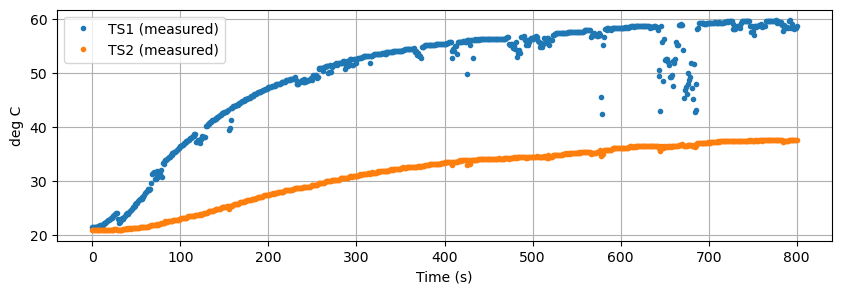
Data was recorded for 800 seconds and saved to a .csv data file. Some noise and data dropouts are evident in the data. The data file is accessible at the link given in the code cell below.
The challenge is to develop a first-principles models that reproduces the system measured response shown below.
import pandas as pd
import matplotlib.pyplot as plt

data_file = "https://raw.githubusercontent.com/jckantor/cbe30338-book/main/notebooks/data/tclab-data-example.csv"
data = pd.read_csv(data_file)
data = data.set_index("Time")
data.head()
| T1 | T2 | Q1 | Q2 | |
|---|---|---|---|---|
| Time | ||||
| 0.00 | 21.543 | 20.898 | 50.0 | 0.0 |
| 1.00 | 21.543 | 20.898 | 50.0 | 0.0 |
| 2.01 | 21.543 | 20.898 | 50.0 | 0.0 |
| 3.01 | 21.543 | 20.931 | 50.0 | 0.0 |
| 4.00 | 21.543 | 20.931 | 50.0 | 0.0 |
The Pandas library includes a highly functional method for plotting data.
data.plot(y=["T1", "T2"], figsize=(10, 3), grid=True, ylabel="deg C", xlabel="Time (s)", linestyle="",marker=".")
plt.legend(["TS1 (measured)", "TS2 (measured)"])
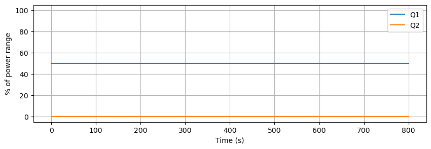
data.plot(y=["Q1", "Q2"], figsize=(10, 3), grid=True, ylabel="% of power range", ylim=(-5, 105), xlabel="Time (s)")
plt.show()
2.5.2. Two-State Model#
For this model we no longer assume the heater and sensor are at the same temperature. To account for differing temperatures, we introduce \(T_{H,1}\) to denote the temperature of heater one and \(T_{S,1}\) to denote the temperature of the corresponding sensor. We further assume the sensor exchanges heat only with the heater, and heat transfer to the surroundings is dominated by the heat sink attached to the heater.
This motivates a model
where \(C^H_p\) and \(C^S_p\) are the heat capacities of the heater and sensor, respectively, and \(U_b\) is a new heat transfer coefficient characterizing the exchange of heat between the heater and sensor. Where the temperature measured and recorded by the Arduino is given by
The following cell creates a simulation of heater/sensor combination.
import numpy as np
from scipy.integrate import solve_ivp
import pandas as pd

# known parameters
T_amb = 21             # deg C
alpha = 0.00016        # watts / (units P1 * percent U1)
P1 = 200               # P1 units

# adjustable parameters
CpH = 5                # joules/deg C
CpS = 1                # joules/deg C
Ua = 0.05              # watts/deg C
Ub = 0.05              # watts/deg C

# initial conditions
TH1 = T_amb
TS1 = T_amb
IC = [TH1, TS1]

# input values
U1 = 50                # steady state value of u1 (percent)

# extract data from experiment
t_expt = data.index

def tclab_ode(param):
    # unpack the adjustable parameters
    CpH, CpS, Ua, Ub = param

    # model solution
    def deriv(t, y):
        TH1, TS1 = y
        dTH1 = (-Ua*(TH1 - T_amb) + Ub*(TS1 - TH1) + alpha*P1*U1)/CpH
        dTS1 = Ub*(TH1 - TS1)/CpS
        return [dTH1, dTS1]

    soln = solve_ivp(deriv, [min(t_expt), max(t_expt)], IC, t_eval=t_expt)

    # create dataframe with predictions
    pred = pd.DataFrame(columns=["Time"])
    pred["Time"] = t_expt
    pred = pred.set_index("Time")

    # report the model temperatures
    pred["TH1"] = soln.y[0]
    pred["TS1"] = soln.y[1]

    # report the prediced measurement
    pred["T1"] = pred["TS1"]

    return pred

pred = tclab_ode(param=[CpH, CpS, Ua, Ub])
pred
| TH1 | TS1 | T1 | |
|---|---|---|---|
| Time | |||
| 0.00 | 21.000000 | 21.000000 | 21.000000 |
| 1.00 | 21.316847 | 21.007816 | 21.007816 |
| 2.01 | 21.630650 | 21.030852 | 21.030852 |
| 3.01 | 21.935475 | 21.067561 | 21.067561 |
| 4.00 | 22.231957 | 21.115691 | 21.115691 |
| ... | ... | ... | ... |
| 796.00 | 52.948664 | 52.946492 | 52.946492 |
| 797.01 | 52.949058 | 52.947023 | 52.947023 |
| 798.01 | 52.949466 | 52.947455 | 52.947455 |
| 799.00 | 52.949892 | 52.947773 | 52.947773 |
| 800.01 | 52.950354 | 52.947967 | 52.947967 |
801 rows × 3 columns
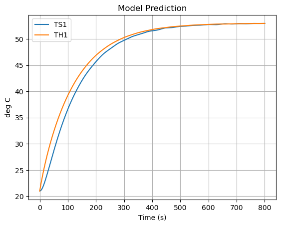
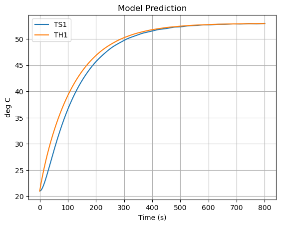
pred.plot(y=["TS1","TH1"],grid=True, ylabel="deg C", title="Model Prediction", xlabel="Time (s)")
plt.show()
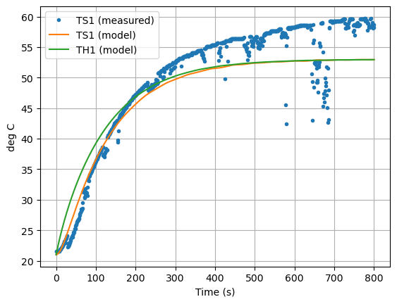
Now let’s compare the predicted measurement to the actual measurement. How did we do?
ax = data.plot(y=["T1"], grid=True, linestyle="", marker=".")
ax = pred.plot(ax=ax,y=["TS1", "TH1"], ylabel="deg C", xlabel="Time (s)", grid=True)
plt.legend(["TS1 (measured)","TS1 (model)", "TH1 (model)"])
plt.show()
2.5.3. State Space Model#
Our two-state model for the temperature control lab is given by
The initial steady state is \(T_{amb}\). So let’s write the dependent variables as excursions from the ambient temperature.
Then divide by the heat capacities.
The two-state model can be rewritten using vectors to collect the states, inputs, measurable outputs, and arrays to collect the coefficients of the differential equations.
In other words, we can write the temperature control lab model as a state-space model
where the state space variables are the deviations of temperature from the ambient \(T_{amb}\)
and parameters are embedded in the arrays
By using the notation and techniques of linear algebra, state-space models provide a compact means of representing complex systems. This example consists of \(m=1\) inputs, \(n=2\) states, and \(p=1\) outputs.
The following is an example of printing formatting.
print(f"pi = {np.pi:8.3f} isn't that nice")
pi = 3.142 isn't that nice
print(f"{Ua=} watts/deg C")
Ua=0.05 watts/deg C
import numpy as np
from scipy.integrate import solve_ivp
import  pandas as pd

# known parameters
T_amb = 21             # deg C
alpha = 0.00016        # watts / (units P1 * percent U1)
P1 = 200               # P1 units

# adjustable parameters
CpH = 5                # joules/deg C
CpS = 1                # joules/deg C
Ua = 0.05              # watts/deg C
Ub = 0.05              # watts/deg C

# array parameters
A = np.array([[-(Ua + Ub)/CpH, Ub/CpH], [Ub/CpS, -Ub/CpS]])
B = np.array([[alpha*P1/CpH], [0]])
C = np.array([[0, 1]])

print(f"\n{A=}")
print(f"\n{B=}")
print(f"\n{C=}")
A=array([[-0.02,  0.01],
       [ 0.05, -0.05]])

B=array([[0.0064],
       [0.    ]])

C=array([[0, 1]])
# input values
U1 = 50                # steady state value of u1 (percent)
def u(t):
    return np.array([U1])

# extract data from experiment
t_expt = data.index

def tclab_ss(A, B, C):

    IC = [0, 0]

    # model solution
    def deriv(t, x):
        dxdt = A @ x + B @ u(t)
        return dxdt

    soln = solve_ivp(deriv, [min(t_expt), max(t_expt)], IC, t_eval=t_expt)

    # create dataframe with predictions
    pred = pd.DataFrame(columns=["Time"])
    pred["Time"] = t_expt
    pred = pred.set_index("Time")

    # get the state variables
    pred["x1"] = soln.y[0]
    pred["x2"] = soln.y[1]

    pred["y"] = pred["x2"]

    # convert back to model temperatures
    pred["TH1"] = pred["x1"] + T_amb
    pred["TS1"] = pred["x2"] + T_amb

    # report the predicated measurement
    pred["T1"] = pred["TS1"]

    return pred

pred = tclab_ss(A, B, C)

pred.head()
| x1 | x2 | y | TH1 | TS1 | T1 | |
|---|---|---|---|---|---|---|
| Time | ||||||
| 0.00 | 0.000000 | 0.000000 | 0.000000 | 21.000000 | 21.000000 | 21.000000 |
| 1.00 | 0.316847 | 0.007816 | 0.007816 | 21.316847 | 21.007816 | 21.007816 |
| 2.01 | 0.630651 | 0.030850 | 0.030850 | 21.630651 | 21.030850 | 21.030850 |
| 3.01 | 0.935462 | 0.067618 | 0.067618 | 21.935462 | 21.067618 | 21.067618 |
| 4.00 | 1.231700 | 0.116765 | 0.116765 | 22.231700 | 21.116765 | 21.116765 |
pred.plot(y=["TS1","TH1"],grid=True, ylabel="deg C", title="Model Prediction", xlabel="Time (s)")
plt.show()
2.5.4. “Least Squares” Model Fitting#
Fitting a model to data is a basic task in engineering, science, business, and a foundation of modern data sciences. For engineers the goal is to validate hypotheses about how a device works, then to enable simulation and design. In the data science model fitting may be almost completely empirical using black box models to develop predictive models of complex systems.
In this case we wish to find values for a small number of parameters that cause a model to replicate a measured response. One common measure of fit is the sum of sum of squares of residual difference between the model and data. For residuals modeled as independent and identically distributed random variables from a Gaussian distribution, minimizing the sum of squares has a strong theoretical foundation. So strong, in fact, the term “least squares” has become synonomous with model fitting and regression.
The SciPy library includes a well-developed function scipy.optimize.least_squares for this purpose. The name is a misnomoer because the function allows other common “loss” functions in addition to sum of squares. The simplest use of least_squares is to provide a function that, given values for the unknown parameters, creates a vector of residuals between a model and data.
This is demonstrated below.
# Try your hand at trial and error data fitting
# adjustable parameters
CpH = 5 # joules/deg C
CpS = 1 # joules/deg C
Ua = 0.04 # watts/deg C
Ub = 0.04 # watts/deg C
A = np.array([[-(Ua + Ub)/CpH, Ub/CpH], [Ub/CpS, -Ub/CpS]])
B = np.array([[alpha*P1/CpH], [0]])
C = np.array([[0, 1]])
pred = tclab_ss(A, B, C)
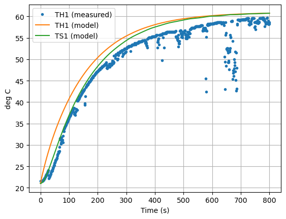
ax = data["T1"].plot(grid=True, linestyle="", marker=".")
pred.plot(ax=ax, y=["TH1","TS1"],xlabel="Time (s)", ylabel="deg C", grid=True)
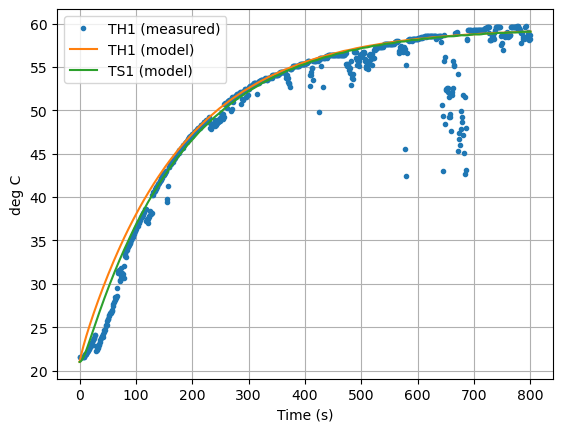
plt.legend(["TH1 (measured)", "TH1 (model)", "TS1 (model)"])
plt.show()
def pred_err(p):
CpH, CpS, Ua, Ub = p
# array parameters
A = np.array([[-(Ua + Ub)/CpH, Ub/CpH], [Ub/CpS, -Ub/CpS]])
B = np.array([[alpha*P1/CpH], [0]])
C = np.array([[0, 1]])
pred = tclab_ss(A, B, C)
return pred["T1"] - data["T1"]
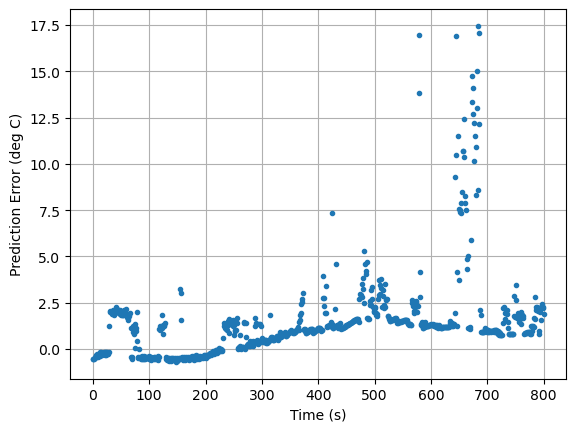
pred_err([5.8, 1, 0.04, 0.045]).plot(xlabel="Time (s)", ylabel="Prediction Error (deg C)", grid=True, linestyle="", marker=".")
<Axes: xlabel='Time (s)', ylabel='Prediction Error (deg C)'>
from scipy.optimize import least_squares
results = least_squares(pred_err, [8, 1, 0.05, 0.05], loss="cauchy")
CpH, CpS, Ua, Ub = results.x
print(f"CpH = {CpH}, CpS = {CpS}, Ua = {Ua}, Ub = {Ub}")
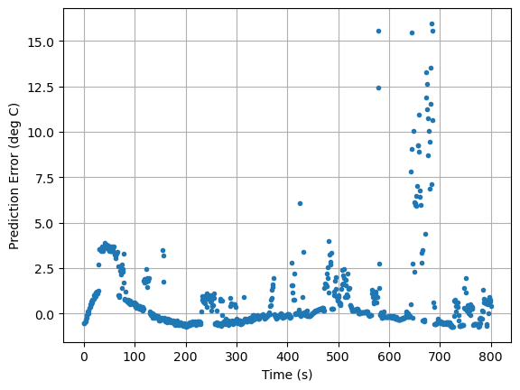
pred_err([CpH, CpS, Ua, Ub]).plot(xlabel="Time (s)", ylabel="Prediction Error (deg C)", grid=True, linestyle="", marker=".")
CpH = 5.2280012374973746, CpS = 1.9897188470054918, Ua = 0.04157103899328196, Ub = 0.21309849232002476
<Axes: xlabel='Time (s)', ylabel='Prediction Error (deg C)'>
A = np.array([[-(Ua + Ub)/CpH, Ub/CpH], [Ub/CpS, -Ub/CpS]])
B = np.array([[alpha*P1/CpH], [0]])
C = np.array([[0, 1]])

pred = tclab_ss(A, B, C)
ax = data["T1"].plot(linestyle="", marker=".")
ax = pred.plot(ax=ax, y=["TH1","TS1"],xlabel="Time (s)", ylabel="deg C", grid=True)
plt.legend(["TH1 (measured)", "TH1 (model)", "TS1 (model)"])
plt.show()
Choosing a Loss Function
Consult the documentation page scipy.optimize.least_squares. Modify the regression to use alternative loss functions including soft_l1, huber, cauchy and arctan.
Which gives the best result?
From the documentation, why is the fit better?
How much of difference does it make it estimated model parameters?
from scipy.optimize import least_squares

# Test different loss functions
loss_functions = ['linear', 'soft_l1', 'huber', 'cauchy', 'arctan']
results_dict = {}
parameters_dict = {}

print("Testing different loss functions:\n")
print(f"{'Loss Function':<15} {'Cost':<15} {'CpH':<10} {'CpS':<10} {'Ua':<10} {'Ub':<10}")
print("=" * 75)

for loss in loss_functions:
    try:
        # Use appropriate f_scale for robust loss functions
        if loss == 'linear':
            results = least_squares(pred_err, [8, 1, 0.05, 0.05], loss=loss, max_nfev=5000)
        else:
            # For robust losses, use a larger f_scale to avoid numerical issues
            results = least_squares(pred_err, [8, 1, 0.05, 0.05], loss=loss, f_scale=1.0, max_nfev=5000)

        results_dict[loss] = results
        CpH, CpS, Ua, Ub = results.x
        parameters_dict[loss] = (CpH, CpS, Ua, Ub)

        print(f"{loss:<15} {results.cost:<15.6f} {CpH:<10.4f} {CpS:<10.4f} {Ua:<10.4f} {Ub:<10.4f}")
    except Exception as e:
        print(f"{loss:<15} {'ERROR':<15} {str(e)[:40]}")

print("\n" + "=" * 75)
Testing different loss functions:

Loss Function   Cost            CpH        CpS        Ua         Ub
===========================================================================
linear          1836.366811     2.8988     2.0130     0.0436     0.0369
/opt/anaconda3/envs/controls/lib/python3.10/site-packages/scipy/optimize/_lsq/least_squares.py:221: RuntimeWarning: overflow encountered in square
  z = (f / f_scale) ** 2
soft_l1 80.712081 6.4103 0.7020 0.0418 0.0766
---------------------------------------------------------------------------
ValueError                                Traceback (most recent call last)
Cell In[15], line 18
     15     results = least_squares(pred_err, [8, 1, 0.05, 0.05], loss=loss)
     16 else:
     17     # For robust losses, f_scale represents the noise level; typically set between 0.01-0.1
---> 18     results = least_squares(pred_err, [8, 1, 0.05, 0.05], loss=loss, f_scale=0.1)
     20 results_dict[loss] = results
     21 CpH, CpS, Ua, Ub = results.x

File /opt/anaconda3/envs/controls/lib/python3.10/site-packages/scipy/optimize/_lsq/least_squares.py:941, in least_squares(fun, x0, jac, bounds, method, ftol, xtol, gtol, x_scale, loss, f_scale, diff_step, tr_solver, tr_options, jac_sparsity, max_nfev, verbose, args, kwargs)
    937     result = call_minpack(fun_wrapped, x0, jac_wrapped, ftol, xtol, gtol,
    938                           max_nfev, x_scale, diff_step)
    940 elif method == 'trf':
--> 941     result = trf(fun_wrapped, jac_wrapped, x0, f0, J0, lb, ub, ftol, xtol,
    942                  gtol, max_nfev, x_scale, loss_function, tr_solver,
    943                  tr_options.copy(), verbose)
    945 elif method == 'dogbox':
    946     if tr_solver == 'lsmr' and 'regularize' in tr_options:

File /opt/anaconda3/envs/controls/lib/python3.10/site-packages/scipy/optimize/_lsq/trf.py:119, in trf(fun, jac, x0, f0, J0, lb, ub, ftol, xtol, gtol, max_nfev, x_scale, loss_function, tr_solver, tr_options, verbose)
    112 def trf(fun, jac, x0, f0, J0, lb, ub, ftol, xtol, gtol, max_nfev, x_scale,
    113         loss_function, tr_solver, tr_options, verbose):
    114     # For efficiency, it makes sense to run the simplified version of the
    115     # algorithm when no bounds are imposed. We decided to write the two
    116     # separate functions. It violates the DRY principle, but the individual
    117     # functions are kept the most readable.
    118     if np.all(lb == -np.inf) and np.all(ub == np.inf):
--> 119         return trf_no_bounds(
    120             fun, jac, x0, f0, J0, ftol, xtol, gtol, max_nfev, x_scale,
    121             loss_function, tr_solver, tr_options, verbose)
    122     else:
    123         return trf_bounds(
    124             fun, jac, x0, f0, J0, lb, ub, ftol, xtol, gtol, max_nfev, x_scale,
    125             loss_function, tr_solver, tr_options, verbose)

File /opt/anaconda3/envs/controls/lib/python3.10/site-packages/scipy/optimize/_lsq/trf.py:499, in trf_no_bounds(fun, jac, x0, f0, J0, ftol, xtol, gtol, max_nfev, x_scale, loss_function, tr_solver, tr_options, verbose)
    497 step = d * step_h
    498 x_new = x + step
--> 499 f_new = fun(x_new)
    500 nfev += 1
    502 step_h_norm = norm(step_h)

File /opt/anaconda3/envs/controls/lib/python3.10/site-packages/scipy/optimize/_lsq/least_squares.py:830, in least_squares.<locals>.fun_wrapped(x)
    829 def fun_wrapped(x):
--> 830     return np.atleast_1d(fun(x, *args, **kwargs))

Cell In[12], line 10, in pred_err(p)
      7 B = np.array([[alpha*P1/CpH], [0]])
      8 C = np.array([[0, 1]])
---> 10 pred = tclab_ss(A, B, C)
     11 return pred["T1"] - data["T1"]

Cell In[9], line 26, in tclab_ss(A, B, C)
     23 pred = pred.set_index("Time")
     25 # get the state variables
---> 26 pred["x1"] = soln.y[0]
     27 pred["x2"] = soln.y[1]
     29 pred["y"] = pred["x2"]

File /opt/anaconda3/envs/controls/lib/python3.10/site-packages/pandas/core/frame.py:4311, in DataFrame.__setitem__(self, key, value)
   4308     self._setitem_array([key], value)
   4309 else:
   4310     # set column
-> 4311     self._set_item(key, value)

File /opt/anaconda3/envs/controls/lib/python3.10/site-packages/pandas/core/frame.py:4524, in DataFrame._set_item(self, key, value)
   4514 def _set_item(self, key, value) -> None:
   4515     """
   4516     Add series to DataFrame in specified column.
   4517
   (...)
   4522     ensure homogeneity.
   4523     """
-> 4524     value, refs = self._sanitize_column(value)
   4526     if (
   4527         key in self.columns
   4528         and value.ndim == 1
   4529         and not isinstance(value.dtype, ExtensionDtype)
   4530     ):
   4531         # broadcast across multiple columns if necessary
   4532         if not self.columns.is_unique or isinstance(self.columns, MultiIndex):

File /opt/anaconda3/envs/controls/lib/python3.10/site-packages/pandas/core/frame.py:5266, in DataFrame._sanitize_column(self, value)
   5263     return _reindex_for_setitem(value, self.index)
   5265 if is_list_like(value):
-> 5266     com.require_length_match(value, self.index)
   5267 arr = sanitize_array(value, self.index, copy=True, allow_2d=True)
   5268 if (
   5269     isinstance(value, Index)
   5270     and value.dtype == "object"
   (...)
   5273     # TODO: Remove kludge in sanitize_array for string mode when enforcing
   5274     # this deprecation

File /opt/anaconda3/envs/controls/lib/python3.10/site-packages/pandas/core/common.py:573, in require_length_match(data, index)
    569 """
    570 Check the length of data matches the length of the index.
    571 """
    572 if len(data) != len(index):
--> 573     raise ValueError(
    574         "Length of values "
    575         f"({len(data)}) "
    576         "does not match length of index "
    577         f"({len(index)})"
    578     )

ValueError: Length of values (557) does not match length of index (801)