Lab 3: Relay (On-Off) Control

Lab 3: Relay (On-Off) Control#

Your Name:

In this lab assignment you will implement relay control for the Temperature Control Laboratory. The class website explains the Python interface to the TCLab in more detail. Your main tasks are:

Use numerical simulation to tune your controller (Exercise 0)
Implement and test a relay control for the heater/sensor system
Implement and test a relay control to track a complex setpoint (dark chocolate tempering)

Spring 2025 TODO List#

Add numeric simulation of dark chocolate tempering
Save all results to csv files
Add code to calculate the average absolute tracking error and root mean squared tracking error for the simulations and two exercises

Excercise 0. Simulation#

This exercise is due BEFORE the start of lab. It is a pre-lab assignment. Your task:

Read the entire lab assigment. If you have a question, post to Canvas.
Create a plot showing the setpoints described in Excercise 1.
On paper (or a tablet), write down the system of differential equations for the TCLab with the simple relay controller described in Exercise 1. Include in your model the intial conditions for each state. For simplity, you can set the deadband to zero, i.e., \(d=0\). This makes it easier to use solve_ivp.
Hint: You can assume your two TCLab channels are identical and there is no interaction between the channels. It will be an imperfect model, but you have enough information to build it. Here are some ideas from a legacy page on the class website.
Using Python, numerically simulate the system of differential equations. Use the TCLab model parameters you estimated in Lab 2 for your personal TCLab hardware.

### Create a plot showing the setpoints described in Exercise 1

# modify these setpoints to change with time
def SP1_simple(t):
    """Set point definition for T1
    Arguments:
        t: time (s)
    Returns:
        set point of T1
    """
    return 40

def SP2_simple(t):
    """Set point definition for T2
    Arguments:
        t: time (s)
    Returns:
        set point of T2
    """
    return 35

# Add your solution here

import matplotlib.pyplot as plt
import numpy as np

# Add your solution here

### Simulate differential equations for the TCLab system plus relay controller

# Add your solution here

Write a few observations about your simulation result. (Recommendation: Write 3 to 5 bullet points where each bullet point is one idea, expressed in one or two sentences.)

Answer:

Exercise 1. Simple Relay Control for TC Lab#

Create a relay controller subject to the following requirements:

Simultaneous control of sensor temperatures \(T_1\) and \(T_2\) to setpoints 35 and 40 °C, respectively. The setpoints return to 25 °C at t = 300.
Use a tolerance value \(d\) of 0.5 °C.
Set the minimum and maximum values of the heater to 0 and 100%, respectively.
Set ‘lab.P1’ and ‘lab.P2’ to 200 to be consistent with prior labs.
Run the experiment for at least 500 seconds.
Show the results of an experiment in which the setpoints are adjusted accordingly.

Debug Your Implementation with the TCLab Digital Twin#

The tclab library includes a simulation-mode/digital twin. This allows you to debug your controller code BEFORE using your hardware. This is really helpful as the digital twin does not require anytime to cool down.

Here is the code to use the digital twin:

TCLab = setup(connected=False, speedup=5)

Setting connected=False enables the simulation-mode (a.k.a., digital twin). When connected=False, you can also use the speedup argument to speed-up the simulation. Again, this is super helpful for debugging your code.

With great power comes great responsibility. While the digital twin mode is increadibly helpful, it is very easy to forget to set connected=True again before running the actual experiments in the lab. In later Exercises, you must run the experiments on your TCLab hardware. It is important you tripple check connected=True.

Below is some starter code.

# As a first step, let's verify the sample code runs

from tclab import TCLab, clock, Historian, Plotter, setup

''' Important note about the 'setup' function:
connected=False is used for the simulation.
connected=True is used to connect to the real device.
speedup=5 can be used to run the simulation at 5x real time.
'''
TCLab = setup(connected=False, speedup=5)


# relay controller
def relay(SP, d=1, Umin=0, Umax=100):
    """Relay controller definition
    Arguments:
        SP: set point function
        d: set point tolerance
        Umin: minimum heater output (%) 
        Umax: maximum heater output (%)
    Returns:
        none
    """
    #start with the heater off
    U = 0
    #while the simulation is active (t<tfinal)
    while True:
        t, T = yield U
        #When T is below the set point, turn on heater
        if T < SP(t) - d/2:
            U = Umax
        #When T is above the set point, turn off heater
        if T > SP(t) + d/2:
            U = Umin

# create a single control loop for T1
controller1 = relay(SP1_simple)
controller1.send(None)

# This started code only implements a controller for T1
# What do you need to change to implement a controller for T2 too?

#simulate with TCLab
t_final = 60 # change this to 500 seconds for the actual experiment
t_step = 1
with TCLab() as lab:
    sources = [("T1", lambda: lab.T1), ("T2", lambda: lab.T2),
               ("SP1", lambda: SP1(t)), ("SP2", lambda: SP2(t)),
               ("Q1", lab.Q1), ("Q2", lab.Q2)]
    #load historian
    h = Historian(sources)
    #load plotter
    p = Plotter(h, t_final, layout=(("T1", "SP1"), ("T2", "SP2"), ("Q1", "Q2")))
    #While time is less than tfinal
    for t in clock(t_final, t_step):
        ## Controller for T1
        # This starter code only manipulates U1 to control T1.
        # Your specifications also give a setpoint for T2
        T1 = lab.T1
        # Send the controller time and T1 data
        U1 = controller1.send([t, T1])
        lab.Q1(U1)

        ## Controller for T2
        # What do you need to change to implement a controller for T2 too?

        ## Read data and update plot
        p.update()

Verify your Device is at Ambient Temperature#

# Verify your device has cooled back to ambient
tfinal = 30 #seconds

# perform experiment
with TCLab() as lab:
    #Set power to 0
    lab.U1 = 0
    lab.U2 = 0
    #load historian 
    h = Historian(lab.sources)
    #Load plotter
    p = Plotter(h, tfinal)
    #While time is less than tfinal
    for t in clock(tfinal):
        #Read data and update plot
        p.update(t)

# Copy the code you implemented and debugged above

TCLab = setup(connected=True)

# Add your solution here

# Need to save results to a csv file

Discussion#

Write a 1 to 3 sentences to answer each of the following questions.

Q1 Describe the shape of the temperature profiles (time-series) for the excrise 1 experiment. Are these shapes expected?

Answer:

Q2 Speculate about why T1 overshoots the setpoint more than T2 in the excerise 1 experiment.

Answer:

Q3 Describe the shape of the temperature profiles (time-series) for the excrise 1 experiment. Are these shapes expected?

Answer:

Exercise 2. Tempering Chocolate#

We now want to create a rely controller that matches the temperature profile for tempering chocolate.

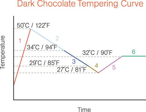
Temperature 1 specifications:

Start from ambient.
Reach 50 °C at 3 minutes, 27 °C at 7 minutes, return to 32 °C at 8 minutes, and hold until 10 minutes.
The goal is follow the linear ramp between setpoints as closely as possible.

Temperature 2 specifications:

Start from ambient, ramp, and then hold at 30 °C.

Hints:

Modify SP1 to linearly interpolate the set point as a function of time.

Plot the Described Temperature Profile#

# Complete these function to define the setpoints for T1 and T2
def SP1_chocolate(t):
    """Set point definition for T1
    Arguments:
        t: time (s)
    Returns:
        set point of T1
    """
    # Add your solution here

def SP2_chocolate(t):
    """Set point definition for T2
    Arguments:
        t: time (s)
    Returns:
        set point of T2
    """
    # Add your solution here

# Make a plot of the setpoints to verify your setpoint functions
# are correct.

# Add your solution here

Verify TCLab is at Ambient Temperature#

TCLab = setup(connected=True)

# Add your solution here

Perform Experiment with TCLab Hardware#

# Copy your code from above and modify to match the specifications

# You may optionally set connected=False to debug your code
# If you do, you MUST set it back to connected=True before running the experiment
# You should also rerun the code block above to verify your TCLab is at ambient temperature
# BEFORE running this experiment
TCLab = setup(connected=True)

# Add your solution here

Discussion#

Q1 In the cholcate tempering simulation, how many times does each heater transitions from (a) one to off and (b) off to on? Fill in the table below.

Sensor	On to Off	Off to On
T1
T2

Answer:

Q2 Descibe the shape of the T1 and T2 timeseries for the excerise 2 experiment. How do the T1 and T2 profiles relate to the on/off and off/on transitions for Q1 and Q2?

Answer:

Exercise 3. Comparing Simulations and Hardward Performance.#

Simulate Performance of Relay Controller for Dark Cholocate Tempering#

Create a Function to Quantify Controller Performance#

Performance of Simulated Controller for Simple Experiment#

Performance of TCLab Device for Simple Experiment#

Performance of Simulated Controller for Chocolate Experiment#

Performance of TCLab Device for Chocolate Experiment#

Summary#

Concluding Discussion#

The following questions tie together the Exercises throughout the lab. Please write 1 to 3 sentences per prompt.

Q1 How can we reduce the oscillations in these experiments? Propose at least one idea and provide reasoning for why it could work.

Answer:

Consider the following feedback diagram from the first day of class:

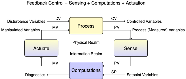
Identify the variables in each of the categories for our temperature control lab.

Maninpulated Variable(s):

Answer:

Controlled Variable(s):

Answer:

Process/Measured Variable(s):

Answer:

Set Point Variable(s):

Answer:

Disturbance Variable(s):

Answer:

Bonus Exercise (Extra Credit)#

Using your code from Lab 2 as a starting point, reestimate the parameters in the four-state TCLab model (\(T_S\) and \(T_H\) for both channels). Perform simultanous nonlinear regression with four datasets:

Step test (Lab 1)
Sine test (Lab 2)
Simple Relay On/Off Experiment (Lab 3)
Chocolate Tempering Relay On/Off Experiment (Lab 3)

You should start by deriving the four state model on paper. You may need to perform multi-start initialization. Include time-series plots, analysis of the residuals, and quantification of uncertainty, similar to Lab 2. How much did your parameter estimates change compared to Lab 2? How much did the parameter uncertainty decrease (or increase)? Do the results make sense and why?

# Add your solution here
        return [dT1H, dT1S, dT2H, dT2S]

    soln = solve_ivp(deriv, [min(t_expt), max(t_expt)], [T_amb, T_amb], t_eval=t_expt)

    T1H = soln.y[0]
    T1S = soln.y[1]
    T2H = soln.y[2]
    T2S = soln.y[3]

    if plot:
        # Plot the temperature data and heat power
        plt.figure()
        plt.subplot(2,1,1)
        plt.plot(t_expt, data['T1'], 'ro', label='Measured $T_S$')
        plt.plot(t_expt, T1S, 'b-', label='Predicted $T_{S1}$')
        plt.plot(t_expt, T1H, 'g-', label='Predicted $T_{H1}$')
        plt.plot(t_expt, T2S, 'r-', label='Predicted $T_{S2}$')
        plt.plot(t_expt, T2H, 'p-', label='Predicted $T_{H2}$')
        plt.ylabel('Temperature (degC)')
        plt.legend()
        plt.subplot(2,1,2)
        plt.plot(t_expt, data['Q1'], 'g-', label='Heater 1')
        plt.plot(t_expt, data['Q2'], 'p-', label='Heater 2')
        plt.ylabel('Heater (%)')
        plt.legend()
        plt.xlabel('Time (sec)')
        plt.title(plot_title)
        plt.tight_layout()
        plt.show()

    return TS

# Test your function with the data and initial parameters
TS = tclab_model4(data, [0.1, 0.2, 4, 0.1], plot=True)

### END SOLUTION

Common Mistakes#

Not using the correct kernel (for the controls environment with TCLab installed)
Not setting up controller #2 (This includes assigning T2 and Q2 in the simulation code)
When switching to connected=True most got errors if they did not restart the kernel and clear all the cells output
Trying to create their own linear interpolation function, just use np.interp

Declarations#

TCLab Hardware: Did you use the same TCLab device for Labs 1, 2, and 3? If not, please provide details here. These labs are designed to use the same hardware throughout the semester. Please keep this in mind as you answer the discussion questions, especially when comparing the simulated to actual performance.

Collaboration: If you worked with any classmates, please give their names here. Describe the nature of the collaboration.

Generative AI: If you used any Generative AI tools, please elaborate here.

Reminder: The written discussions responses must be in your own words. Many of these questions ask about your specific results or are open-ended questions with many reasonable answers. Thus we expect unique responses, analyses, and ideas.

We may use writing analysis software to check for overly similar written responses. You are responsible for reviewing the colaboration policy outlined in the class syllabus to avoid violations of the honor code.

Lab 3: Relay (On-Off) Control

Contents

Lab 3: Relay (On-Off) Control#

Spring 2025 TODO List#

Excercise 0. Simulation#

Exercise 1. Simple Relay Control for TC Lab#

Debug Your Implementation with the TCLab Digital Twin#

Verify your Device is at Ambient Temperature#

Discussion#

Exercise 2. Tempering Chocolate#

Plot the Described Temperature Profile#

Verify TCLab is at Ambient Temperature#

Perform Experiment with TCLab Hardware#

Discussion#

Exercise 3. Comparing Simulations and Hardward Performance.#

Simulate Performance of Relay Controller for Dark Cholocate Tempering#

Create a Function to Quantify Controller Performance#

Performance of Simulated Controller for Simple Experiment#

Performance of TCLab Device for Simple Experiment#

Performance of Simulated Controller for Chocolate Experiment#

Performance of TCLab Device for Chocolate Experiment#

Summary#

Concluding Discussion#

Bonus Exercise (Extra Credit)#

Common Mistakes#

Declarations#