6.5. Implementing Predictive Control#
The goal of this notebook is to demonstrate an implementation of predictive control.
6.5.1. Model#
Once agaiin will use the two-state model for a single heater/sensor assembly to demonstrate the key elements of this notebook.
The model is recast into linear state space form as
where
and
The following cell creates values for the model parameters.
%matplotlib inline
import matplotlib.pyplot as plt
import numpy as np
import cvxpy as cp

# parameter estimates.
alpha = 0.00016       # watts / (units P * percent U1)
P1 = 200              # P units
P2 = 100              # P units
Ua = 0.050            # heat transfer coefficient from heater to environment
CpH = 2.2             # heat capacity of the heater (J/deg C)
CpS = 1.9             # heat capacity of the sensor (J/deg C)
Ub = 0.021            # heat transfer coefficient from heater to sensor

# state space model
A = np.array([[-(Ua + Ub)/CpH, Ub/CpH], [Ub/CpS, -Ub/CpS]])
Bu = np.array([[alpha*P1/CpH], [0]])     # single column
Bd = np.array([[Ua/CpH], [0]])           # single column
C = np.array([[0, 1]])                   # single row
6.5.2. Control Objective#
An optimal control policy minimizes the differences
where \(SP(t)\) is a setpoint, subject to constraints
initial conditions
where \(T_{amb}(t)\) is a possibly time-varying disturbance.
# estimates of future behavior
Tamb = 20
SP = 45
6.5.3. Assumptions Need to Use Optimization for Real-Time Feedback#
Predictive control is a strategy that uses optimization for feedback control. The basic concept is to solve an optimization problem at every time step utilizing all of the information available up to that point in time. The key assumptions are:
The current value of the setpoint will be held constant into the future.
The current estimate of any disturbances will be constant into the future.
The state at the current time is available from a state estimator.
Assumptions 1 and 2 are obviously very strong statements about the future. But in the absence of additional information, these assumptions are about the best we can expect.
6.5.4. Bare Bones Event Loop#
Borrowing from notebook 4.6, we start the process of implementing predictive control by starting with an implementation of a simpler strategy (relay control) that includes a state observer. With that framework in place, we will show what modifications are need to implement predictive control.
Note: This code has been cut and pasted from earlier notebooks, but with some edits for brevity and clarity.
6.5.4.1. Relay Control#
The relay controller is an instance of a Python generator that is sent values of the setpoint and process variable, and yields values for a manipulated variable. Each instance of the relay controller is initialized with minimum and maximum values of the manipulated variable. Later we will be replacing the relay control with a predictive control.
# Relay Control
def relay(MV_min, MV_max):
    MV = MV_min
    while True:
        # yield manipulated variable. Wait for message from the
        # event with updated setpoint and process variable measurement.
        SP, PV = yield MV
        MV = MV_min if PV >= SP else MV_max
6.5.4.2. Observer#
Given current values of the manipulated input, the sensor measurement, and estimated disturbance sent from the event loop, the observer updates the state estimate
def tclab_observer(L, t_prev=0, x=[Tamb, Tamb], d=[Tamb]):
    while True:
        # yield current state estimate. Wait for message information
        # needed to update the state estimate for the next time step
        t, U, T_sensor, Tamb = yield x

        # prediction
        x = x + (t - t_prev)*(A@x + Bu@[U] + Bd@[Tamb])

        # correction
        x = x - (t - t_prev)*L@(C@x - np.array([T_sensor]))
        t_prev = t
from tclab import setup, clock, Historian, Plotter

t_final = 300
t_step = 2

# create and initialize a controller instance
controller = relay(0, 100)
U1 = next(controller)

# create and initialize an observer instance
L = np.array([[0.4], [0.2]])
observer = tclab_observer(L)
Th, Ts = next(observer)

# execute the event loop
TCLab = setup(connected=False, speedup=10)
with TCLab() as lab:
    h = Historian([('SP', lambda: SP),
                   ('T1', lambda: T1),
                   ('U1', lambda: U1),
                   ('Th', lambda: Th),
                   ('Ts', lambda: Ts),
                   ('Tamb', lambda: Tamb)])
    p = Plotter(h, t_final, layout=[['T1','Ts','Th', 'SP', 'Tamb'], ['U1']])
    for t in clock(t_final, t_step):
        T1 = lab.T1
        Th, Ts = observer.send([t, U1, T1, Tamb])
        U1 = controller.send([SP, Ts])
        lab.Q1(U1)
        p.update(t)
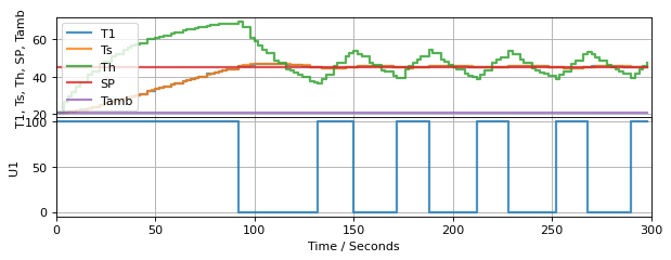
TCLab Model disconnected successfully.
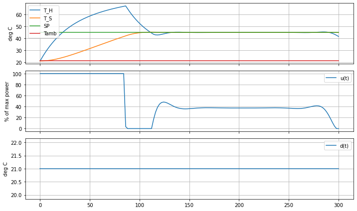
6.5.5. Feedforward Optimization#
As a preliminary step, we first create a CVXPY model that that computes a feedforward control policy given values for the setpoint \(SP\), disturbance \(T_{amb}\), and the current state. This code was cut-and-pasted from a previous notebook, with modifications to use the values SP and Tamb defined in this notebook.
t_horizon = 300
dt = 2
n = round(t_horizon/dt)
t_grid = np.linspace(0, t_horizon, n+1)

# add $u$ as a decision variable
u = {t: cp.Variable(1, nonneg=True) for t in t_grid}
x = {t: cp.Variable(2) for t in t_grid}
y = {t: cp.Variable(1) for t in t_grid}

# least-squares optimization objective
objective = cp.Minimize(sum((SP - y[t])**2 for t in t_grid))

model = [x[t] == x[t-dt] + dt*(A@x[t-dt] + Bu@u[t-dt] + Bd@[Tamb]) for t in t_grid[1:]]
output = [y[t] == C@x[t] for t in t_grid]
inputs = [u[t] <= 100 for t in t_grid]
IC = [x[0] == np.array([Tamb, Tamb])]

problem = cp.Problem(objective,  model + IC + output + inputs)
problem.solve()

# display solution
fix, ax = plt.subplots(3, 1, figsize=(10,6), sharex=True)
ax[0].plot(t_grid, [x[t][0].value  for t in t_grid], label="T_H")
ax[0].plot(t_grid, [x[t][1].value  for t in t_grid], label="T_S")
ax[0].plot(t_grid, [SP for t in t_grid], label="SP")
ax[0].plot(t_grid, [Tamb for t in t_grid], label="Tamb")
ax[0].set_ylabel("deg C")
ax[0].legend()
ax[1].plot(t_grid, [u[t].value for t in t_grid], label="u(t)")
ax[1].set_ylabel("% of max power")
ax[2].plot(t_grid, [Tamb for t in t_grid], label="d(t)")
ax[2].set_ylabel("deg C")
for a in ax:
    a.grid(True)
    a.legend()
plt.tight_layout()
6.5.5.1. A Predictive Controller#
The next step is to encapsulate the feedforward control computation into a generator that can be run from the event loop each time new information becomes available.
The warm_start option tells CVXPY to use results from the prior soluton to update the current solution. Not every solver offers this feature, but when they do it can often lead to a signficant speedup of the computations.
def predictive_control(t_horizon=300, dt=2):
    # create time grid
    n = round(t_horizon/dt)
    t_grid = np.linspace(0, t_horizon, n+1)

    # create decision variables and all parts of the model
    # that do not depend on information from the event loop
    u = {t: cp.Variable(1, nonneg=True) for t in t_grid}
    x = {t: cp.Variable(2) for t in t_grid}
    y = {t: cp.Variable(1) for t in t_grid}
    output = [y[t] == C@x[t] for t in t_grid]
    inputs = [u[t] <= 100 for t in t_grid]

    MV = 0
    while True:
        # yield MV, then wait for new information to update MV
        SP, Th, Ts, Tamb = yield MV
        objective = cp.Minimize(sum((y[t]-SP)**2 for t in t_grid))
        model = [x[t] == x[t-dt] + dt*(A@x[t-dt] + Bu@u[t-dt] + Bd@[Tamb]) for t in t_grid[1:]]
        IC = [x[0] == np.array([Th, Ts])]
        problem = cp.Problem(objective,  model + IC + output + inputs)
        problem.solve(warm_start=True)
        MV = u[0].value[0]
6.5.6. Testing the Predictive Controller#
Let’s put the predictive controller to work. Note that the speedup factor the simulation has been changed. This is needed to accomodate the far more intensive calculations that are taking place at each time step.
t_final = 300
t_step = 2

# create a controller instance
controller = predictive_control(dt=t_step)
U1 = next(controller)

# create estimator instance
L = np.array([[0.4], [0.2]])
observer = tclab_observer(L)
Th, Ts = next(observer)

# execute the event loop
TCLab = setup(connected=False, speedup=5)
with TCLab() as lab:
    h = Historian([('SP', lambda: SP),
                   ('T1', lambda: T1),
                   ('U1', lambda: U1),
                   ('Th', lambda: Th),
                   ('Ts', lambda: Ts),
                   ('Tamb', lambda: Tamb)])
    p = Plotter(h, t_final, layout=[['T1','Ts','Th', 'SP', 'Tamb'], ['U1']])
    for t in clock(t_final, t_step):
        T1 = lab.T1
        Th, Ts = observer.send([t, U1, T1, Tamb])
        U1 = controller.send([SP, Th, Ts, Tamb])
        lab.Q1(U1)
        p.update(t)
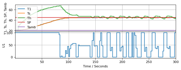
TCLab Model disconnected successfully.
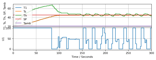
Study Question: Compare the closed-loop response of the simulation where the control policy is continually updated to the previous feedforward control calculation. List a few ways they are the similar? List a few ways they are different.
6.5.7. Lab Assignment 9#
6.5.7.1. Exercise 1. Improving the Predictive Controller#
While we appear to have a working controller, there are some problems revealed by the simulation that need to be fixed before attempting to to use this on real hardware. The major issues are:
The controller is sensitive to minor modeling errors. The control action makes large changes in response to small measurement errors which would not be a good thing for real hardware.
There is little guidance on how to choose the time horizon and time step for the predictive control calculations.
The predictive control calculations are slow.
Let’s consider the first of these issues. The predictive control given above minimizes the following objective:
This objective includes no mention of the control variable \(u\) which means the optimizer can call for large changes in \(u\) with no penalty. This can be modified.
where \(0 \leq \alpha \leq 1\) tells us how much weight to put on each objective. When \(\alpha=0\) the only goal is to keep the setpoint error small. When \(\alpha=1\) the only goal is to minimize changes in the manipulable input. Clearly we want to find a compromise between these two competing goals.
In the cells below, copy and paste the code for the predictive control and the closed-loop simulation for the two state model. Name the new control generator my_predictive_control. Make the following modifications:
Implement the modified objective described above. Include
alphaas a named parameter in the control generator with a default value of 0. Verify that you can reproduce the results given above for \(alpha=0\). Then test for values of \(alpha\) equal to 0.01, 0.1, and 0.5. Based on your engineering judgemet, which value would you choose for use on your hardware? Why?To speed up the control computations, modify the predictive controller to use larger time steps in the calculation (for this step, don’t change the time step in the event loop, just the time step in the controller). Try values of 5 and 10 seconds. What do you observe? Again, using your engineering judgement, choose a value to implement on your hardware.
Next, change the value of the time step in the event loop. Start by doubling to 4 seconds. Keep doubling. Pick a time step for the event loop for hardware use that doesn’t overly compromise control performance.
For your assignment, you only need to show the final simulation result of these tuning procedures.
def my_predictive_control(t_horizon=300, dt=2):
    # create time grid
    n = round(t_horizon/dt)
    t_grid = np.linspace(0, t_horizon, n+1)

    # create decision variables and all parts of the model
    # that do not depend on information from the event loop
    u = {t: cp.Variable(1, nonneg=True) for t in t_grid}
    x = {t: cp.Variable(2) for t in t_grid}
    y = {t: cp.Variable(1) for t in t_grid}
    output = [y[t] == C@x[t] for t in t_grid]
    inputs = [u[t] <= 100 for t in t_grid]

    MV = 0
    while True:
        # yield MV, then wait for new information to update MV
        SP, Th, Ts, Tamb = yield MV
        objective = cp.Minimize(sum((y[t]-SP)**2 for t in t_grid))
        model = [x[t] == x[t-dt] + dt*(A@x[t-dt] + Bu@u[t-dt] + Bd@[Tamb]) for t in t_grid[1:]]
        IC = [x[0] == np.array([Th, Ts])]
        problem = cp.Problem(objective,  model + IC + output + inputs)
        problem.solve(warm_start=True)
        MV = u[0].value[0]
t_final = 300
t_step = 2

# create a controller instance
controller = predictive_control(dt=t_step)
U1 = next(controller)

# create estimator instance
L = np.array([[0.4], [0.2]])
observer = tclab_observer(L)
Th, Ts = next(observer)

# execute the event loop
TCLab = setup(connected=False, speedup=5)
with TCLab() as lab:
    h = Historian([('SP', lambda: SP),
                   ('T1', lambda: T1),
                   ('U1', lambda: U1),
                   ('Th', lambda: Th),
                   ('Ts', lambda: Ts),
                   ('Tamb', lambda: Tamb)])
    p = Plotter(h, t_final, layout=[['T1','Ts','Th', 'SP', 'Tamb'], ['U1']])
    for t in clock(t_final, t_step):
        T1 = lab.T1
        Th, Ts = observer.send([t, U1, T1, Tamb])
        U1 = controller.send([SP, Th, Ts, Tamb])
        lab.Q1(U1)
        p.update(t)
TCLab Model disconnected successfully.
6.5.7.2. Exercise 2. Predictive control of the four state model.#
Using the results of the first exercise, now modify the your code to accomodate the complete four state model of the TCLab hardware.
Targeting setpoints of 45 and 35 degrees for the sensor temperatures, test your results in simulation.
Modify the code to control the heater temperatures to those same setpoints. Do you need to modify your controller tuning?
For this exercise, you only need to show the final simulation result.
6.5.7.3. Exercise 3. Putting it all together.#
For the final exercise, apply the results of Exercise 2 to your actual device hardware. Run the experiment for at least 600 seconds. How did you do?
6.5.7.4. Exercise 4. Do something nice for yourself.#
Congratulations on your newly minted expertise! If you got this far, then you have successfully implemented multivariable model predictive control on real hardware. That’s an outstanding accomplishment for any engineer, and gives you the conceptual and practical framework to understand many of the contemporary applications of advanced process control.
If you want validation, just Google “Model predictive control of” and add a topic of interest to you.