Collocation Points and Runge-Kutta Coefficients

Prepared by: Prof. Alexander Dowling

This notebook is the computational companion to the collocation lecture. Rather than copying the collocation points and Butcher coefficients out of a table, we derive them: the collocation points come out of an orthogonality condition, the basis polynomials come out of a symbolic integral, and the coefficient table comes out of evaluating that integral. Every number is then checked against the published values.

import sys

if "google.colab" in sys.modules:
    !wget "https://raw.githubusercontent.com/ndcbe/optimization/main/notebooks/helper.py"
    import helper

    helper.easy_install()
else:
    sys.path.insert(0, "../")
    import helper
helper.set_plotting_style()

import numpy as np
import sympy as sym
import matplotlib.pyplot as plt

# The normalized coordinate on one finite element, tau in [0, 1]
tau = sym.symbols("tau", real=True)

Notebook context¶

This notebook follows Chapter 10 of Biegler (2010). It assumes the quadrature background in Dynamic Optimization with Collocation and Pyomo.DAE and the Runge-Kutta notation in Numeric Integration for DAEs.

Three questions, answered in order:

Where do the basis polynomials $\bar\ell_j(\tau)$ and $\Omega_j(\tau)$ come from?
Where do the collocation points $\tau_j$ come from, for each of the three families?
How do those two produce the Runge-Kutta (Butcher) coefficients $a_{j,k}$ and $b_k$ ?

The two Lagrange bases¶

On finite element $i$ we write $t = t_{i-1} + h_i \tau$ with $\tau \in [0,1]$ . There are two Lagrange bases in play, and they are not the same object.

The state is interpolated through $K+1$ points, including $\tau_0 = 0$ :

z^K(t) = \sum_{j=0}^K \ell_j(\tau) z_{ij}, \qquad \ell_j(\tau) = \prod_{\substack{k=0 \\ k \neq j}}^K \frac{\tau - \tau_k}{\tau_j - \tau_k}.

(1)

The derivative is interpolated through only the $K$ collocation points, and $\tau_0 = 0$ is not one of them:

\bar\ell_j(\tau) = \prod_{\substack{k=1 \\ k \neq j}}^K \frac{\tau - \tau_k}{\tau_j - \tau_k}, \qquad \Omega_j(\tau) = \int_0^{\tau} \bar\ell_j(\tau')\, d\tau', \qquad j = 1, \ldots, K,

(2)

which gives the Runge-Kutta representation of the state,

z^K(t) = z_{i-1} + h_i \sum_{j=1}^K \Omega_j(\tau)\, \dot{z}_{ij}.

(3)

Important

$\bar\ell_j$ under the integral, not $\ell_j$ . The printed text of Biegler (2010) defines $\Omega_j(\tau) = \int_0^{\tau} \ell_j(\tau')\,d\tau'$ with the $(K+1)$ -point basis. That is a typo, corrected in errata2.pdf (Chapter 10, correction 1). The correct integrand is the $K$ -point basis $\bar\ell_j$ .

The tell is the degree. $\bar\ell_j$ has degree $K-1$ , so $\Omega_j$ has degree $K$ --- which is what the book says a few lines earlier. With $\ell_j$ (degree $K$ ) under the integral $\Omega_j$ would come out degree $K+1$ , and the collocation equations would no longer match. We check both degrees numerically below, so the erratum is a computation here rather than a claim.

Order and degree. $\ell_j$ and $\Omega_j$ both have degree $K$ , but $\ell_j$ has $K+1$ free coefficients while $\Omega_j(0)=0$ leaves only $K$ . Thus the lecture’s use of order counts free coefficients rather than degree.

Building $\bar\ell_j$ and $\Omega_j$ symbolically¶

Both definitions are products and one integral, so sympy can carry them exactly. We keep the collocation points as exact numbers (rationals and surds) all the way through, and convert to floating point only at the very end.

def lagrange_basis(points, j):
    """Lagrange basis polynomial through `points`, equal to 1 at points[j] and 0 elsewhere.

    Arguments:
        points: list of interpolation points (sympy expressions)
        j: index of the point where this basis polynomial equals 1

    Returns:
        sympy expression in tau
    """
    expr = sym.Integer(1)
    for k, tau_k in enumerate(points):
        if k != j:
            expr *= (tau - tau_k) / (points[j] - tau_k)
    return sym.expand(expr)


def omega_basis(points):
    """Runge-Kutta basis polynomials Omega_j(tau) = int_0^tau ellbar_j(tau') dtau'.

    Arguments:
        points: the K collocation points tau_1, ..., tau_K (tau_0 = 0 is NOT included)

    Returns:
        list of K sympy expressions in tau
    """
    return [
        sym.expand(sym.integrate(lagrange_basis(points, j), (tau, 0, tau)))
        for j in range(len(points))
    ]

Where the collocation points come from¶

The exact solution of $\dot z = f(z,t)$ on one element is

z(t_i) = z(t_{i-1}) + \int_{t_{i-1}}^{t_i} f(z(t), t)\, dt,

(4)

and collocation replaces that integral with a $K$ -point quadrature rule. A rule with $K$ free nodes and $K$ free weights has $2K$ degrees of freedom, so the best possible rule is exact for polynomials of degree $2K-1$ . Theorem 10.1 of Biegler says the nodes that achieve it are the roots of a degree- $K$ polynomial orthogonal on $[0,1]$ .

Constraining an endpoint to be a node spends a degree of freedom and buys a property. That is the whole difference between the three families:

Family	Fixed nodes	Free nodes	Weight $w(\tau)$	Jacobi $(\alpha, \beta)$	Truncation error
Gauss-Legendre	none	$K$	1	$(0, 0)$	$O(h^{2K})$
Gauss-Radau	$\tau_K = 1$	$K-1$	$(1-\tau)$	$(1, 0)$	$O(h^{2K-1})$
Gauss-Lobatto	$\tau_1 = 0$ , $\tau_K = 1$	$K-2$	$\tau(1-\tau)$	$(1, 1)$	$O(h^{2K-2})$

The free nodes are the roots of the monic polynomial $P_n(\tau)$ of degree $n$ (the number of free nodes) satisfying the Gauss-Jacobi orthogonality condition

\int_0^1 w(\tau)\, \tau^m\, P_n(\tau)\, d\tau = 0, \qquad m = 0, \ldots, n-1.

(5)

We build $P_n$ by Gram-Schmidt on the monomials $1, \tau, \tau^2, \ldots$ using that weighted inner product. This is not the numerically preferred route for large $K$ --- the Golub-Welsch eigenvalue algorithm is --- but it is exact, it is short, and it makes the orthogonality condition visible instead of hiding it in a library call.

def monic_orthogonal(n, weight):
    """Monic degree-n polynomial orthogonal to all lower degrees on [0, 1].

    Gram-Schmidt on the monomials under the inner product
    <p, q> = int_0^1 weight(tau) p(tau) q(tau) dtau.

    Arguments:
        n: degree of the polynomial to return
        weight: sympy expression in tau, the Gauss-Jacobi weight function

    Returns:
        sympy expression in tau
    """
    basis = []
    for m in range(n + 1):
        p = tau**m
        for q in basis:
            numer = sym.integrate(weight * p * q, (tau, 0, 1))
            denom = sym.integrate(weight * q * q, (tau, 0, 1))
            p = p - (numer / denom) * q
        basis.append(sym.expand(sym.simplify(p)))
    return basis[n]


# Fixed nodes and Gauss-Jacobi weight for each family
FAMILIES = {
    "Gauss-Legendre": {"fixed": [], "weight": sym.Integer(1)},
    "Gauss-Radau": {"fixed": [sym.Integer(1)], "weight": 1 - tau},
    "Gauss-Lobatto": {
        "fixed": [sym.Integer(0), sym.Integer(1)],
        "weight": tau * (1 - tau),
    },
}


def collocation_points(family, K):
    """Collocation points tau_1 < ... < tau_K on [0, 1], derived from orthogonality.

    Arguments:
        family: one of the keys of FAMILIES
        K: number of collocation points

    Returns:
        sorted list of K exact sympy expressions
    """
    fixed = FAMILIES[family]["fixed"]
    weight = FAMILIES[family]["weight"]
    n_free = K - len(fixed)
    assert n_free >= 0, f"{family} needs K >= {len(fixed)}"

    if n_free > 0:
        P = monic_orthogonal(n_free, weight)
        free = sym.Poly(P, tau).all_roots()
    else:
        free = []

    return sorted([sym.simplify(r) for r in free] + fixed, key=float)

Reproducing Biegler Table 10.1¶

The table below is generated, not transcribed. Compare it to Table 10.1 on p. 292 of Biegler (2010).

COLLOCATION_POINTS = {}

for family in FAMILIES:
    K_min = len(FAMILIES[family]["fixed"])
    print(f"\n{family}")
    for K in range(max(K_min, 1), 6):
        points = collocation_points(family, K)
        COLLOCATION_POINTS[(family, K)] = points
        values = "  ".join(f"{float(p):.6f}" for p in points)
        print(f"  K = {K}:  {values}")


Gauss-Legendre
  K = 1:  0.500000
  K = 2:  0.211325  0.788675
  K = 3:  0.112702  0.500000  0.887298

  K = 4:  0.069432  0.330009  0.669991  0.930568

  K = 5:  0.046910  0.230765  0.500000  0.769235  0.953090

Gauss-Radau
  K = 1:  1.000000
  K = 2:  0.333333  1.000000
  K = 3:  0.155051  0.644949  1.000000
  K = 4:  0.088588  0.409467  0.787659  1.000000

  K = 5:  0.057104  0.276843  0.583590  0.860240  1.000000

Gauss-Lobatto
  K = 2:  0.000000  1.000000
  K = 3:  0.000000  0.500000  1.000000
  K = 4:  0.000000  0.276393  0.723607  1.000000
  K = 5:  0.000000  0.172673  0.500000  0.827327  1.000000

Two of these values are quoted directly in the lecture, so we assert them. If a solver or sympy version ever changes an answer here, the notebook fails loudly instead of quietly publishing a wrong table.

# Gauss-Radau, K = 3 -- the points you type into a model (Biegler Table 10.1, p. 292)
radau3 = [float(p) for p in COLLOCATION_POINTS[("Gauss-Radau", 3)]]
assert np.allclose(radau3, [0.155051, 0.644949, 1.0], atol=1e-6), radau3

# Gauss-Legendre, K = 3 -- note the largest root is NOT 1, which is why the
# Legendre continuity equation needs Omega_k(1) rather than a_{Nc,k}
legendre3 = [float(p) for p in COLLOCATION_POINTS[("Gauss-Legendre", 3)]]
assert np.isclose(max(legendre3), 0.887298, atol=1e-6), legendre3

# Exact (radical) forms, for the record
print("Gauss-Radau,     K = 3:", COLLOCATION_POINTS[("Gauss-Radau", 3)])
print("Gauss-Legendre,  K = 3:", COLLOCATION_POINTS[("Gauss-Legendre", 3)])
print("Gauss-Lobatto,   K = 3:", COLLOCATION_POINTS[("Gauss-Lobatto", 3)])

Gauss-Radau,     K = 3: [2/5 - sqrt(6)/10, sqrt(6)/10 + 2/5, 1]
Gauss-Legendre,  K = 3: [1/2 - sqrt(15)/10, 1/2, sqrt(15)/10 + 1/2]
Gauss-Lobatto,   K = 3: [0, 1/2, 1]

Building the coefficient table¶

With the points in hand, the Runge-Kutta (Butcher) coefficients are just evaluations of $\Omega_k$ :

c_j = \tau_j, \qquad a_{j,k} = \Omega_k(\tau_j), \qquad b_k = \Omega_k(1).

(6)

That is the entire content of the tableau. Nothing else is fitted or tuned.

def butcher_tableau(family, K, digits=None):
    """Derive the Runge-Kutta (Butcher) coefficients for a collocation family.

    Arguments:
        family: one of the keys of FAMILIES
        K: number of collocation points (stages)
        digits: if given, round the collocation points to this many digits before
            building the basis. The symbolic route is exact but the expressions
            blow up past K = 4, where the roots are no longer radicals. Pass
            digits=25 to keep the algebra fast; leave it None for exact results.

    Returns:
        c: list of K collocation points
        A: K-by-K nested list, A[j][k] = Omega_k(tau_j)
        b: list of K quadrature weights, b[k] = Omega_k(1)
        Omega: the K basis polynomials, for plotting and degree checks
    """
    c = COLLOCATION_POINTS.get((family, K)) or collocation_points(family, K)
    if digits is not None:
        c = [sym.Float(p.evalf(digits), digits) for p in c]
    Omega = omega_basis(c)

    # Deliberately no simplify() here: the entries stay exact either way, and
    # simplifying nested radicals at K > 3 is slow. Simplify at the point of use.
    A = [[Omega[k].subs(tau, c[j]) for k in range(K)] for j in range(K)]
    b = [Omega[k].subs(tau, 1) for k in range(K)]

    return c, A, b, Omega


def print_tableau(family, K):
    """Print the Butcher tableau in the usual c | A / b layout."""
    c, A, b, _ = butcher_tableau(family, K)
    print(f"{family}, K = {K}")
    for j in range(K):
        row = "  ".join(f"{float(a):>12.8f}" for a in A[j])
        print(f"  {float(c[j]):.8f} |{row}")
    print("  " + "-" * (12 + 14 * K))
    print("             |" + "  ".join(f"{float(w):>12.8f}" for w in b))


print_tableau("Gauss-Radau", 3)

Gauss-Radau, K = 3
  0.15505103 |  0.19681548   -0.06553543    0.02377097
  0.64494897 |  0.39442431    0.29207341   -0.04154875
  1.00000000 |  0.37640306    0.51248583    0.11111111
  ------------------------------------------------------
             |  0.37640306    0.51248583    0.11111111

This is the 3-stage Radau IIA tableau. In exact arithmetic the entries are

c_radau3, A_radau3, b_radau3, Omega_radau3 = butcher_tableau("Gauss-Radau", 3)

for j in range(3):
    for k in range(3):
        print(f"a_({j + 1},{k + 1}) = {sym.radsimp(sym.simplify(A_radau3[j][k]))}")
for k in range(3):
    print(f"b_{k + 1}     = {sym.radsimp(sym.simplify(b_radau3[k]))}")

a_(1,1) = 11/45 - 7*sqrt(6)/360
a_(1,2) = 37/225 - 169*sqrt(6)/1800
a_(1,3) = -2/225 + sqrt(6)/75

a_(2,1) = 37/225 + 169*sqrt(6)/1800
a_(2,2) = 7*sqrt(6)/360 + 11/45
a_(2,3) = -sqrt(6)/75 - 2/225
a_(3,1) = 4/9 - sqrt(6)/36

a_(3,2) = sqrt(6)/36 + 4/9
a_(3,3) = 1/9
b_1     = 4/9 - sqrt(6)/36
b_2     = sqrt(6)/36 + 4/9
b_3     = 1/9

Verification against the published tableaus¶

The 3-stage Radau IIA, Gauss (Legendre) and Lobatto IIIA tableaus are standard. We check every entry symbolically, so a match is exact rather than to six digits.

sqrt6 = sym.sqrt(6)
sqrt15 = sym.sqrt(15)

# Radau IIA, 3 stages (Hairer & Wanner; equivalently Biegler Example 10.2)
A_radau_published = [
    [
        sym.Rational(11, 45) - 7 * sqrt6 / 360,
        sym.Rational(37, 225) - 169 * sqrt6 / 1800,
        -sym.Rational(2, 225) + sqrt6 / 75,
    ],
    [
        sym.Rational(37, 225) + 169 * sqrt6 / 1800,
        sym.Rational(11, 45) + 7 * sqrt6 / 360,
        -sym.Rational(2, 225) - sqrt6 / 75,
    ],
    [
        sym.Rational(4, 9) - sqrt6 / 36,
        sym.Rational(4, 9) + sqrt6 / 36,
        sym.Rational(1, 9),
    ],
]
b_radau_published = A_radau_published[2]

# Gauss (Legendre), 3 stages
A_gauss_published = [
    [
        sym.Rational(5, 36),
        sym.Rational(2, 9) - sqrt15 / 15,
        sym.Rational(5, 36) - sqrt15 / 30,
    ],
    [
        sym.Rational(5, 36) + sqrt15 / 24,
        sym.Rational(2, 9),
        sym.Rational(5, 36) - sqrt15 / 24,
    ],
    [
        sym.Rational(5, 36) + sqrt15 / 30,
        sym.Rational(2, 9) + sqrt15 / 15,
        sym.Rational(5, 36),
    ],
]
b_gauss_published = [sym.Rational(5, 18), sym.Rational(4, 9), sym.Rational(5, 18)]

# Lobatto IIIA, 3 stages
A_lobatto_published = [
    [sym.Integer(0), sym.Integer(0), sym.Integer(0)],
    [sym.Rational(5, 24), sym.Rational(1, 3), -sym.Rational(1, 24)],
    [sym.Rational(1, 6), sym.Rational(2, 3), sym.Rational(1, 6)],
]
b_lobatto_published = [sym.Rational(1, 6), sym.Rational(2, 3), sym.Rational(1, 6)]

PUBLISHED = {
    "Gauss-Radau": (A_radau_published, b_radau_published),
    "Gauss-Legendre": (A_gauss_published, b_gauss_published),
    "Gauss-Lobatto": (A_lobatto_published, b_lobatto_published),
}

for family, (A_ref, b_ref) in PUBLISHED.items():
    _, A_computed, b_computed, _ = butcher_tableau(family, 3)
    for j in range(3):
        for k in range(3):
            assert (
                sym.simplify(A_computed[j][k] - A_ref[j][k]) == 0
            ), f"{family}: a_({j + 1},{k + 1}) disagrees"
    for k in range(3):
        assert (
            sym.simplify(b_computed[k] - b_ref[k]) == 0
        ), f"{family}: b_{k + 1} disagrees"
    print(f"{family:16s} K = 3: A and b match the published tableau exactly.")

Gauss-Radau      K = 3: A and b match the published tableau exactly.
Gauss-Legendre   K = 3: A and b match the published tableau exactly.
Gauss-Lobatto    K = 3: A and b match the published tableau exactly.

Two structural identities hold for any collocation method, and they are cheap to check. They are also the two mistakes that are easiest to make when typing a tableau by hand.

for family in FAMILIES:
    for K in range(max(len(FAMILIES[family]["fixed"]), 1), 6):
        c, A, b, _ = butcher_tableau(family, K, digits=25)

        # Row sums: sum_k a_{j,k} = c_j, because sum_k Omega_k(tau) = tau
        for j in range(K):
            assert np.isclose(
                float(sum(A[j])), float(c[j])
            ), f"{family} K={K}: row {j + 1}"

        # Weights sum to one: the quadrature rule reproduces int_0^1 dtau = 1
        assert np.isclose(float(sum(b)), 1.0), f"{family} K={K}: weights"

print("Row sums equal c and weights sum to 1 for every family and K = 1 to 5.")

Row sums equal c and weights sum to 1 for every family and K = 1 to 5.

What the tableau names mean¶

Three labels have been used above without explanation: Radau IIA, Lobatto IIIA, and the LAGRANGE-RADAU string you hand to Pyomo.DAE. The Roman numerals are historical names for tableaus. They say nothing about order, and the A in IIA is not A-stability.

The family name fixes the nodes $c_j = \tau_j$ --- that is what the orthogonality condition above derives. The numeral fixes the $A$ matrix built on those nodes, and for one node set more than one $A$ is in circulation.

Radau. The Radau nodes can be anchored at either end of the element. Radau IA anchors $\tau_1 = 0$ ; Radau IIA anchors $\tau_K = 1$ . FAMILIES["Gauss-Radau"] above fixes the node at 1, so everything this notebook prints for Gauss-Radau is Radau IIA --- the same choice scheme="LAGRANGE-RADAU" makes. The endpoint node is what buys stiff decay, which is why the course uses IIA throughout.

Lobatto. The Lobatto nodes fix both endpoints, $\tau_1 = 0$ and $\tau_K = 1$ . Three different methods share those nodes and the same quadrature weights $b$ , and differ only in $A$ :

Label	$A$	A collocation method?
Lobatto IIIA	$a_{jk} = \Omega_k(\tau_j)$ --- the construction in this notebook	yes
Lobatto IIIB	a different $A$ on the same nodes	no
Lobatto IIIC	a different $A$ again, and unlike IIIA it is nonsingular	no

So “the Lobatto method” is ambiguous until the numeral is attached. Everything this notebook computes for Gauss-Lobatto is Lobatto IIIA, because collocation on the Lobatto nodes is IIIA. At $K = 2$ that is the trapezoidal rule.

Which Lobatto is algebraically stable?¶

The distinction decides one row of the comparison table in the collocation lecture, so it is worth pinning down. A Runge-Kutta method is algebraically stable when $b \geq 0$ componentwise and the $K \times K$ matrix

M_{jk} = b_j a_{jk} + b_k a_{kj} - b_j b_k

(7)

is positive semidefinite (Ascher & Petzold, Exercise 4.13, p. 119; Burrage & Butcher, Theorem 2.1). Algebraic stability and AN-stability are the same property --- Burrage & Butcher prove algebraic $\Rightarrow$ AN in their Theorem 3.3, with the converse whenever the $c_j$ are distinct --- which is why the integration lecture introduces AN-stability as “also called algebraic stability”.

Burrage & Butcher (1979) list the algebraically stable classes on printed p. 51: the Gauss methods, Radau IA and Radau IIA, and “the Lobatto IIIC methods”. IIIC is on that list; IIIA is not. Ascher & Petzold Exercise 4.13(c) asks for the other half: show that the trapezoidal method, and hence Lobatto collocation, is not algebraically stable.

The reason is one line of arithmetic, and it holds at every $K$ . The Lobatto node set starts at $\tau_1 = 0$ , and $\Omega_k(0) = 0$ by construction, so the first row of the collocation $A$ vanishes. With $a_{11} = 0$ ,

M_{11} = 2 b_1 a_{11} - b_1^2 = -b_1^2 < 0,

(8)

and a symmetric matrix with a negative diagonal entry is not positive semidefinite. Both halves are checked below.

def stability_matrix(A, b):
    """Algebraic-stability matrix M_{j,k} = b_j a_{j,k} + b_k a_{k,j} - b_j b_k.

    Arguments:
        A: K-by-K nested list of Butcher coefficients
        b: list of K quadrature weights

    Returns:
        sympy Matrix, K by K
    """
    K = len(b)
    return sym.Matrix(
        K, K, lambda j, k: sym.simplify(b[j] * A[j][k] + b[k] * A[k][j] - b[j] * b[k])
    )


# Lobatto IIIA -- i.e. the tableau this notebook derives -- at every K it derives.
print("Lobatto IIIA (collocation on the Lobatto nodes)")
for K in range(2, 6):
    _, A, b, _ = butcher_tableau("Gauss-Lobatto", K, digits=25)
    M = stability_matrix(A, b)
    print(f"  K = {K}:  b_1 = {float(b[0]):.6f}   M_(1,1) = {float(M[0, 0]):+.6f}")
    assert float(M[0, 0]) < 0, f"K={K}: expected a negative M_(1,1)"
    assert np.isclose(float(M[0, 0]), -(float(b[0]) ** 2)), f"K={K}: M_(1,1) != -b_1^2"

print("M_(1,1) = -b_1^2 < 0, so M is not positive semidefinite: not algebraically stable.")

Lobatto IIIA (collocation on the Lobatto nodes)
  K = 2:  b_1 = 0.500000   M_(1,1) = -0.250000
  K = 3:  b_1 = 0.166667   M_(1,1) = -0.027778
  K = 4:  b_1 = 0.083333   M_(1,1) = -0.006944
  K = 5:  b_1 = 0.050000   M_(1,1) = -0.002500
M_(1,1) = -b_1^2 < 0, so M is not positive semidefinite: not algebraically stable.

# Lobatto IIIC, 2 stages -- the tableau printed by Burrage & Butcher, Example 5.4
# (printed p. 56). Same nodes and same weights as Lobatto IIIA at K = 2; only A differs.
b_lobatto2 = [sym.Rational(1, 2), sym.Rational(1, 2)]

A_IIIA_2 = [  # the trapezoidal rule
    [sym.Integer(0), sym.Integer(0)],
    [sym.Rational(1, 2), sym.Rational(1, 2)],
]
A_IIIC_2 = [
    [sym.Rational(1, 2), -sym.Rational(1, 2)],
    [sym.Rational(1, 2), sym.Rational(1, 2)],
]

# The collocation construction gives IIIA, not IIIC. Assert it rather than assume it.
_, A_derived, b_derived, _ = butcher_tableau("Gauss-Lobatto", 2)
for j in range(2):
    for k in range(2):
        assert sym.simplify(A_derived[j][k] - A_IIIA_2[j][k]) == 0, f"a_({j + 1},{k + 1})"
for k in range(2):
    assert sym.simplify(b_derived[k] - b_lobatto2[k]) == 0, f"b_{k + 1}"

for label, A in [("Lobatto IIIA", A_IIIA_2), ("Lobatto IIIC", A_IIIC_2)]:
    M = stability_matrix(A, b_lobatto2)
    eigs = sorted(float(e) for e in M.eigenvals())
    print(f"{label}:  M = {M.tolist()}   eigenvalues = {eigs}")

assert min(float(e) for e in stability_matrix(A_IIIA_2, b_lobatto2).eigenvals()) < 0
assert all(float(e) >= 0 for e in stability_matrix(A_IIIC_2, b_lobatto2).eigenvals())
print("\nSame nodes, same weights: IIIA has a negative eigenvalue, IIIC does not.")

# Stiff decay, the other row of the lecture table: R(infinity) = 1 - b^T A^(-1) 1.
ones = sym.Matrix([1, 1])
R_inf_IIIC = 1 - (sym.Matrix([b_lobatto2]) * sym.Matrix(A_IIIC_2).inv() * ones)[0, 0]
assert sym.simplify(R_inf_IIIC) == 0
assert sym.Matrix(A_IIIA_2).det() == 0  # IIIA's A is singular: R(infinity) is undefined
print("Lobatto IIIC, K = 2:  A is nonsingular and R(infinity) =", sym.simplify(R_inf_IIIC))

Lobatto IIIA:  M = [[-1/4, 0], [0, 1/4]]   eigenvalues = [-0.25, 0.25]
Lobatto IIIC:  M = [[1/4, -1/4], [-1/4, 1/4]]   eigenvalues = [0.0, 0.5]

Same nodes, same weights: IIIA has a negative eigenvalue, IIIC does not.
Lobatto IIIC, K = 2:  A is nonsingular and R(infinity) = 0

Important

Reading the lecture’s comparison table. The collocation lecture prints AN-stable: Lobatto --- no, with a footnote that Lobatto IIIC is algebraically stable, while the integration lecture calls AN-stability “also called algebraic stability”. Both statements are true, and they are about two different tableaus on the same nodes.

The table’s Lobatto column is the collocation method, Lobatto IIIA --- the one derived here, the one whose $A$ has a vanishing first row, and the one Ascher & Petzold Exercise 4.13(c) shows is not algebraically stable. Not AN-stable, and with $A$ singular it has no stiff decay either.
Lobatto IIIC puts a different $A$ on those same nodes. It is algebraically stable, hence AN-stable, and the computation above shows it is stiffly accurate as well. But it is not a collocation method, so neither this notebook nor any of Pyomo.DAE’s LAGRANGE-* schemes produces it.

There is no contradiction: “Lobatto” in that table means IIIA, and it is only IIIC that is algebraically stable.

Why $\bar\ell_j$ and not $\ell_j$ ¶

Here is the erratum, as a computation. Build $\Omega_j$ both ways for Gauss-Radau with $K = 3$ , compare the degrees, and then compare the coefficient tables they produce.

K = 3
points = COLLOCATION_POINTS[("Gauss-Radau", K)]

# Correct: the K-point basis, tau_0 = 0 excluded
Omega_correct = omega_basis(points)

# Incorrect: the (K+1)-point basis, tau_0 = 0 included, as the PRINTED text has it
points_with_zero = [sym.Integer(0)] + list(points)
Omega_wrong = [
    sym.expand(sym.integrate(lagrange_basis(points_with_zero, j), (tau, 0, tau)))
    for j in range(1, K + 1)
]

print(
    "degree of ellbar_j :",
    [sym.degree(lagrange_basis(points, j), tau) for j in range(K)],
)
print(
    "degree of Omega_j (correct, ellbar under the integral):",
    [sym.degree(o, tau) for o in Omega_correct],
)
print(
    "degree of Omega_j (wrong, ell under the integral)     :",
    [sym.degree(o, tau) for o in Omega_wrong],
)

# The book says Omega_j has degree K. Only the corrected definition delivers that.
assert all(sym.degree(o, tau) == K for o in Omega_correct)
assert all(sym.degree(o, tau) == K + 1 for o in Omega_wrong)

degree of ellbar_j : [2, 2, 2]
degree of Omega_j (correct, ellbar under the integral): [3, 3, 3]
degree of Omega_j (wrong, ell under the integral)     : [4, 4, 4]

A_correct = [
    [float(Omega_correct[k].subs(tau, points[j])) for k in range(K)] for j in range(K)
]
A_wrong = [
    [float(Omega_wrong[k].subs(tau, points[j])) for k in range(K)] for j in range(K)
]

print("a_(j,k) from ellbar (correct)      from ell (wrong)")
for j in range(K):
    left = "  ".join(f"{a:>11.8f}" for a in A_correct[j])
    right = "  ".join(f"{a:>11.8f}" for a in A_wrong[j])
    print(f"  j = {j + 1}:  {left}   |  {right}")

print()
print("largest disagreement:", np.max(np.abs(np.array(A_correct) - np.array(A_wrong))))

# Rows 1 and 2 are simply different methods. Do not let this pass silently.
assert not np.allclose(A_correct, A_wrong)

# The LAST row happens to agree, and the reason is worth knowing: the K-point
# Radau rule is exact through degree 2K-2 = 4, and ell_j has degree K = 3, so
# int_0^1 ell_j = sum_m b_m ell_j(tau_m) = b_j. The quadrature weights survive
# the typo even though the interior tableau does not.
assert np.allclose(A_correct[K - 1], A_wrong[K - 1])
print("weights b_k (last row) agree; the interior coefficients do not.")

a_(j,k) from ellbar (correct)      from ell (wrong)
  j = 1:   0.19681548  -0.06553543   0.02377097   |   0.09119686  -0.00510864   0.00117506
  j = 2:   0.39442431   0.29207341  -0.04154875   |   0.47199753   0.24769203  -0.02495283
  j = 3:   0.37640306   0.51248583   0.11111111   |   0.37640306   0.51248583   0.11111111

largest disagreement: 0.10561862178478974
weights b_k (last row) agree; the interior coefficients do not.

Order of accuracy, measured¶

The truncation-error column of the family table is a claim about how many polynomial degrees the quadrature rule integrates exactly. We can measure it: apply $\sum_k b_k f(\tau_k)$ to $f(\tau) = \tau^d$ for increasing $d$ and find the first degree where it stops being exact.

def highest_exact_degree(family, K, max_degree=14):
    """Highest polynomial degree the K-point quadrature rule integrates exactly on [0, 1]."""
    c, _, b, _ = butcher_tableau(family, K, digits=25)
    c_float = np.array([float(p) for p in c])
    b_float = np.array([float(w) for w in b])
    for d in range(max_degree + 1):
        rule = float(np.dot(b_float, c_float**d))
        exact = 1.0 / (d + 1)
        if not np.isclose(rule, exact, rtol=0, atol=1e-12):
            return d - 1
    return max_degree


print(f"{'Family':16s} {'K':>2s} {'exact through degree':>22s} {'expected':>10s}")
for family, expected in [
    ("Gauss-Legendre", lambda K: 2 * K - 1),
    ("Gauss-Radau", lambda K: 2 * K - 2),
    ("Gauss-Lobatto", lambda K: 2 * K - 3),
]:
    for K in range(max(len(FAMILIES[family]["fixed"]), 1), 6):
        d = highest_exact_degree(family, K)
        assert d == expected(K), f"{family} K={K}: got {d}, expected {expected(K)}"
        print(f"{family:16s} {K:2d} {d:22d} {expected(K):10d}")

Family            K   exact through degree   expected
Gauss-Legendre    1                      1          1
Gauss-Legendre    2                      3          3
Gauss-Legendre    3                      5          5
Gauss-Legendre    4                      7          7
Gauss-Legendre    5                      9          9
Gauss-Radau       1                      0          0
Gauss-Radau       2                      2          2
Gauss-Radau       3                      4          4
Gauss-Radau       4                      6          6
Gauss-Radau       5                      8          8
Gauss-Lobatto     2                      1          1
Gauss-Lobatto     3                      3          3
Gauss-Lobatto     4                      5          5
Gauss-Lobatto     5                      7          7

The measured degrees are exactly $2K-1$ , $2K-2$ and $2K-3$ : each fixed endpoint costs one degree of exactness. That is the price paid for Radau’s stiff decay and for Lobatto’s symmetric node set.

Visualizing the basis polynomials¶

$\Omega_j(\tau)$ is the accumulated contribution of collocation point $j$ as we sweep across the element. Reading the plot: every curve starts at zero (that is the $\int_0^\tau$ ), the value at $\tau = \tau_j$ is the tableau entry $a_{j,k}$ , and the value at $\tau = 1$ is the quadrature weight $b_k$ .

fig, axes = plt.subplots(1, 3, figsize=(13, 4), sharey=True)
tau_grid = np.linspace(0, 1, 201)

for ax, family in zip(axes, FAMILIES):
    c, _, b, Omega = butcher_tableau(family, 3)
    c_float = [float(p) for p in c]

    for k, poly in enumerate(Omega):
        f = sym.lambdify(tau, poly, "numpy")
        ax.plot(tau_grid, f(tau_grid), label=rf"$\Omega_{k + 1}$")
        ax.plot(1.0, float(b[k]), marker="o", color=ax.lines[-1].get_color())

    for point in c_float:
        ax.axvline(point, color="gray", linestyle=":", linewidth=1)

    ax.axhline(0, color="black", linewidth=0.8)
    ax.set_title(f"{family}, K = 3")
    ax.set_xlabel(r"$\tau$")

axes[0].set_ylabel(r"$\Omega_k(\tau)$")
axes[0].legend()
plt.tight_layout()
plt.show()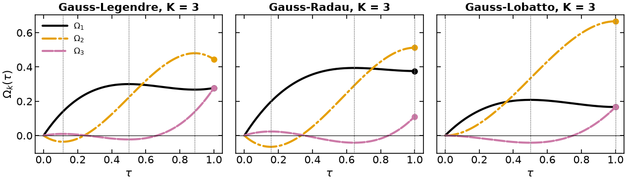

The dotted vertical lines are the collocation points and the markers at $\tau = 1$ are the quadrature weights. Gauss-Lobatto’s first point sits at $\tau_1 = 0$ , which is why its first tableau row is identically zero --- the method evaluates $f$ at the start of the element, where nothing has accumulated yet.

Takeaways¶

The collocation points are not tabulated constants; they are the roots of a shifted Gauss-Jacobi polynomial, and the family is chosen by deciding which endpoints to fix.
The Butcher coefficients are not fitted; they are $a_{j,k} = \Omega_k(\tau_j)$ and $b_k = \Omega_k(1)$ , two evaluations of one integral.
The basis under that integral is $\bar\ell_j$ (the $K$ -point basis), not $\ell_j$ . The degree check above is the fastest way to catch the error.
The Roman numeral names a tableau, not a node set. Collocation on the Lobatto nodes is Lobatto IIIA; Lobatto IIIC is a different $A$ on the same nodes, and it --- not IIIA --- is the algebraically (AN-) stable one.
Each fixed endpoint costs one degree of quadrature exactness, which is the arithmetic behind the $O(h^{2K})$ , $O(h^{2K-1})$ , $O(h^{2K-2})$ column.

In practice Pyomo.DAE builds these coefficients for you --- see Pyomo.DAE: Racing Example Revisited. The point of deriving them once is to know what scheme="LAGRANGE-RADAU" actually selects.

References¶

Biegler, L. T. (2010). Nonlinear Programming: Concepts, Algorithms, and Applications to Chemical Processes. Society for Industrial. 10.1137/1.9780898719383
Burrage, K., & Butcher, J. C. (1979). Stability Criteria for Implicit Runge–Kutta Methods. SIAM Journal on Numerical Analysis, 16(1), 46–57. 10.1137/0716004