Dynamic Optimization with Collocation and Pyomo.DAE

Prepared by: Prof. Alexander Dowling, Molly Dougher (mdoughe6@nd.edu, 2023)

# Install Pyomo and solvers for Google Colab
import sys

if "google.colab" in sys.modules:
    !wget "https://raw.githubusercontent.com/ndcbe/optimization/main/notebooks/helper.py"
    import helper

    helper.easy_install()
else:
    sys.path.insert(0, "../")
    import helper
helper.set_plotting_style()

import numpy as np
import matplotlib.pyplot as plt

Notebook Context¶

Summary information taken from Section 10.1 of Biegler (2010)

As seen in the previous notebooks (2.5 and 2.6), DAEs have a vast range of applications. The goal of this section is to provide the necessary theoretical background to now look at dynamic optimization of an NLP without an embedded DAE solver (Biegler Chapter 10). A multiperiod problem is considered with piecewise polynomial elements representing different states, leading to a discretization that is the same as the Runge-Kutta methods (Biegler Chapter 9).

Quadrature Methods¶

First, the relevant background on quadrature is provided so that it can be applied to the following derivation of collocation methods. These topics are applied to an example in the next section on the website. See the following resources for further information on quadrature methods:

Chapter 9 in Biegler (2010)
Chapter 17 in McClarren (2018)

Main Idea¶

The quadrature rule approximates the integral $I$ with weighted sum of function evaluations:

I := \int_{-1}^{1} f(x) dx \approx \underbrace{\sum_{l=1}^{L} w_l f(x_l)}_{\text{quadrature rule}}

where:

$x_l$ are nodes (also known as abscissas)
$w_l$ are weights
$L$ number of nodes and weights

Central questions:

How to choose nodes and weights?
How does this choice impact approximation error?
How does $L$ impact approximation error?

Recall: The degree and order of a polynomial¶

Consider the polynomial:

p(t) = a_0 + a_1 t + ... + a_K t^K.

(1)

$p(t)$ is said to be of order K+1 as it has K+1 coefficients $a_0, ... a_K$ .

The degree of the polynomial is the highest power with a non-zero coefficient. Thus if $a_K \neq 0$ , then $p(t)$ is degree K.

Gauss-Legendre Quadrature¶

For a specific choice of nodes and weights, the quadrature rule $\sum_{l=1}^{L} w_l f(x_l)$ is exact for integral $I$ if $f(x)$ is a polynomial of degree $2L-1$ or less. This specific case is the optimal (most accurate) rule known as the Gauss-Legendre quadrature.

The weights and nodes are given for $L$ up to 8:

$L$	$x_l$	$w_l$
1	0	2.0
2	±0.5773502691896257645091488	1.0
3	0	0.8888888888888888888888889
	±0.7745966692414833770358531	0.5555555555555555555555556
4	±0.3399810435848562648026658	0.6521451548625461426269361
	±0.8611363115940525752239465	0.3478548451374538573730639
5	0	0.5688888888888888888888889
	±0.5384693101056830910363144	0.4786286704993664680412915
	±0.9061798459386639927976269	0.2369268850561890875142640
6	±0.2386191860831969086305017	0.4679139345726910473898703
	±0.6612093864662645136613996	0.3607615730481386075698335
	±0.9324695142031520278123016	0.1713244923791703450402961
7	0	0.4179591836734693877551020
	±0.4058451513773971669066064	0.3818300505051189449503698
	±0.7415311855993944398638648	0.2797053914892766679014678
	±0.9491079123427585245261897	0.1294849661688696932706114
8	±0.1834346424956498049394761	0.3626837833783619829651504
	±0.5255324099163289858177390	0.3137066458778872873379622
	±0.7966664774136267395915539	0.2223810344533744705443560
	±0.9602898564975362316835609	0.1012285362903762591525314

Why $2L-1$ ?¶

Let $f(x) = a_{2L-1} x^{2L-1} + a_{2L-2} x^{2L-2} + ... + a_{1} x^1 + a_{0}$

Exactness through degree $2L-1$ imposes $2L$ moment equations (one for each monomial $1,x,\ldots,x^{2L-1}$ ). These match the $2L$ unknown node and weight values in an $L$ -point rule. This count motivates the attainable degree; orthogonal-polynomial theory supplies the nodes and proves exactness.

How to determine the nodes and weights?¶

One way to derive the Gauss-Legendre quadrature rules is by looking at the integral generic monomials of degree 0 up to $2L-1$ and setting each equal to the $L$ point Gauss-Legendre quadrature rule:

\begin{align*} \int\limits_{-1}^{1} dx\, a_0 x^0 &= a_0\sum_{l=1}^L w_l x_l^0, \\ \int\limits_{-1}^{1} dx\, a_1 x^1 &= a_1\sum_{l=1}^L w_l x_l^1, \\ & ~~ \vdots \\ \int\limits_{-1}^{1} dx\, a_{2L-1} x^{2L-1} &= a_{2L-1}\sum_{l=1}^L w_l x_l^{2L-1}. \end{align*}

(2)

Notice that the $a_i$ constants cancel out of each equation so they do not matter. This system is $2L$ equations with $L$ weights, $w_l$ , and $L$ nodes, $x_l$ . We could solve these equations to get the weights and nodes, though this is not how it is done in practice generally---this is accomplished by using the theory of orthogonal polynomials.

Code¶

def GLQuad(f, L=8, dataReturn=False):
    """Compute the Gauss-Legendre Quadrature estimate
    of the integral of f(x) from -1 to 1
    Inputs:
    f:   name of function to integrate
    L:   Number of quadrature nodes. Tabulated here for L <= 8;
         larger L falls through to numpy.polynomial.legendre.leggauss.
    dataReturn:   determines whether weights and xs are returned

    Returns:
    G-L Quadrature estimate"""

    # Set bound on L
    assert L >= 1

    # Enumerate over L to define weights and x in each scenario
    if L == 1:
        weights = np.ones(1) * 2
        xs = np.array([0])
    elif L == 2:
        weights = np.ones(2)
        xs = np.array([-np.sqrt(1.0 / 3.0), np.sqrt(1.0 / 3.0)])
    elif L == 3:
        weights = np.array(
            [
                0.8888888888888888888888889,
                0.5555555555555555555555556,
                0.5555555555555555555555556,
            ]
        )
        xs = np.array([0.0, -0.7745966692414833770358531, 0.7745966692414833770358531])
    elif L == 4:
        weights = np.array(
            [
                0.6521451548625461426269361,
                0.6521451548625461426269361,
                0.3478548451374538573730639,
                0.3478548451374538573730639,
            ]
        )
        xs = np.array(
            [
                -0.3399810435848562648026658,
                0.3399810435848562648026658,
                -0.8611363115940525752239465,
                0.8611363115940525752239465,
            ]
        )
    elif L == 5:
        weights = np.array(
            [
                0.5688888888888888888888889,
                0.4786286704993664680412915,
                0.4786286704993664680412915,
                0.2369268850561890875142640,
                0.2369268850561890875142640,
            ]
        )
        xs = np.array(
            [
                0.0,
                -0.5384693101056830910363144,
                0.5384693101056830910363144,
                -0.9061798459386639927976269,
                0.9061798459386639927976269,
            ]
        )
    elif L == 6:
        weights = np.array(
            [
                0.4679139345726910473898703,
                0.4679139345726910473898703,
                0.3607615730481386075698335,
                0.3607615730481386075698335,
                0.1713244923791703450402961,
                0.1713244923791703450402961,
            ]
        )
        xs = np.array(
            [
                -0.2386191860831969086305017,
                0.2386191860831969086305017,
                -0.6612093864662645136613996,
                0.6612093864662645136613996,
                -0.9324695142031520278123016,
                0.9324695142031520278123016,
            ]
        )
    elif L == 7:
        weights = np.array(
            [
                0.4179591836734693877551020,
                0.3818300505051189449503698,
                0.3818300505051189449503698,
                0.2797053914892766679014678,
                0.2797053914892766679014678,
                0.1294849661688696932706114,
                0.1294849661688696932706114,
            ]
        )
        xs = np.array(
            [
                0.0,
                -0.4058451513773971669066064,
                0.4058451513773971669066064,
                -0.7415311855993944398638648,
                0.7415311855993944398638648,
                -0.9491079123427585245261897,
                0.9491079123427585245261897,
            ]
        )
    elif L == 8:
        weights = np.array(
            [
                0.3626837833783619829651504,
                0.3626837833783619829651504,
                0.3137066458778872873379622,
                0.3137066458778872873379622,
                0.2223810344533744705443560,
                0.2223810344533744705443560,
                0.1012285362903762591525314,
                0.1012285362903762591525314,
            ]
        )
        xs = np.array(
            [
                -0.1834346424956498049394761,
                0.1834346424956498049394761,
                -0.5255324099163289858177390,
                0.5255324099163289858177390,
                -0.7966664774136267395915539,
                0.7966664774136267395915539,
                -0.9602898564975362316835609,
                0.9602898564975362316835609,
            ]
        )
    else:  # use numpy's function
        xs, weights = np.polynomial.legendre.leggauss(L)

    # Calculate the quadrature estimate
    quad_estimate = np.sum(weights * f(xs))

    if dataReturn:
        return quad_estimate, weights, xs
    else:
        return quad_estimate

Visualize Weights¶

# Establish L
L = np.arange(1, 15)
# Define a lambda function
f = lambda x: x

# Define the figure
plt.figure(figsize=(4, 4))

# Loop over L
for l in L:
    # Calculate quadrature estimate
    quad_est, weights, xs = GLQuad(f, l, dataReturn=True)
    levels = weights * 0 + l
    plt.scatter(xs, levels, s=weights * 100)

# Format the plot
plt.xlabel("x", fontsize=16, fontweight="bold")
plt.ylabel("L", fontsize=16, fontweight="bold")
plt.tick_params(direction="in", labelsize=15)
plt.title(
    "Gauss-Legendre Quadrature Points\nSize of Point is Weight",
    fontsize=16,
    fontweight="bold",
)
plt.show()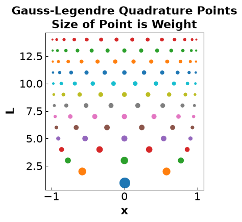

Polynomial Example¶

As a simple demonstration of the Gauss-Legendre quadrature, let’s show that it integrates polynomials of degree $2L-1$ exactly. Consider the integral

\int\limits_{-1}^1 (x+1)^{2L-1}\,dx = \frac{2^{2 L-1}}{L}.

(3)

We can use the GLQuad function to evaluate the error.

L = np.arange(1, 12)
for l in L:

    # Create f
    f = lambda x: (x + 1) ** (2 * l - 1)

    # Evaluate exact (analytic) solution
    integral = 2 ** (2 * l - 1) / l

    # Evaluate quadrature rule
    GLintegral = GLQuad(f, l)

    # Print results
    print(
        "L =",
        l,
        "\t Estimate is",
        GLintegral,
        "Exact value is",
        integral,
        "\nAbs. Relative Error is",
        np.abs(GLintegral - integral) / integral,
    )

L = 1 	 Estimate is 2.0 Exact value is 2.0 
Abs. Relative Error is 0.0
L = 2 	 Estimate is 3.9999999999999996 Exact value is 4.0 
Abs. Relative Error is 1.1102230246251565e-16
L = 3 	 Estimate is 10.666666666666668 Exact value is 10.666666666666666 
Abs. Relative Error is 1.6653345369377348e-16
L = 4 	 Estimate is 31.99999999999999 Exact value is 32.0 
Abs. Relative Error is 3.3306690738754696e-16
L = 5 	 Estimate is 102.39999999999995 Exact value is 102.4 
Abs. Relative Error is 5.551115123125783e-16
L = 6 	 Estimate is 341.33333333333337 Exact value is 341.3333333333333 
Abs. Relative Error is 1.6653345369377348e-16
L = 7 	 Estimate is 1170.2857142857135 Exact value is 1170.2857142857142 
Abs. Relative Error is 5.828670879282072e-16
L = 8 	 Estimate is 4096.000000000003 Exact value is 4096.0 
Abs. Relative Error is 6.661338147750939e-16
L = 9 	 Estimate is 14563.555555555482 Exact value is 14563.555555555555 
Abs. Relative Error is 4.9960036108132044e-15
L = 10 	 Estimate is 52428.79999999968 Exact value is 52428.8 
Abs. Relative Error is 6.106226635438361e-15
L = 11 	 Estimate is 190650.18181818203 Exact value is 190650.18181818182 
Abs. Relative Error is 1.0685896612017132e-15

Generalization¶

We are generally interested in integrals not just over the domain $x\in [-1,1]$ . We’ll now make a function that does Gauss-Legendre quadrature over a general range using the formula

\int_a^b f(x)\,dx = \frac{b-a}{2} \int_{-1}^1 f\left(\frac{b-a}{2}z + \frac{a+b}{2}\right)\,dz.

(4)

def generalGL(f, a, b, L):
    """Compute the Gauss-Legendre Quadrature estimate
    of the integral of f(x) from a to b
    Inputs:
    f:   name of function to integrate
    a:   lower bound of integral
    b:   upper bound of integral
    L:   Number of quadrature nodes (see GLQuad)
    Returns:
    G-L Quadrature estimate"""

    # Set bound on L
    assert L >= 1

    # Define a re-scaled f
    f_rescaled = lambda z: f(0.5 * (b - a) * z + 0.5 * (a + b))

    # Define the integral
    integral = GLQuad(f_rescaled, L)

    # Calculate the G-L quadrature estimate
    return integral * (b - a) * 0.5

Let’s show that this version integrates polynomials of degree $2L-1$ exactly. Consider the integral

\int\limits_{-3}^2 (x+1)^{2L-1}\,dx = \frac{9^L-4^L}{2 L}.

(5)

L = np.arange(1, 12)

# Loop over L to calculate the integral and the G-L estimate
for l in L:
    # Define a lambda function
    f = lambda x: (x + 1) ** (2 * l - 1)
    # Calculate the integral
    integral = (9**l - 4**l) / (2 * l)
    # Calculate the estimate
    GLintegral = generalGL(f, -3, 2, l)
    # Print statement for the error comparison
    print(
        "L =",
        l,
        "\t Estimate is",
        GLintegral,
        "Exact value is",
        integral,
        "\nAbs. Relative Error is",
        np.abs(GLintegral - integral) / integral,
    )

L = 1 	 Estimate is 2.5 Exact value is 2.5 
Abs. Relative Error is 0.0
L = 2 	 Estimate is 16.249999999999996 Exact value is 16.25 
Abs. Relative Error is 2.1862853408003084e-16
L = 3 	 Estimate is 110.83333333333336 Exact value is 110.83333333333333 
Abs. Relative Error is 2.5643647606379557e-16
L = 4 	 Estimate is 788.1249999999999 Exact value is 788.125 
Abs. Relative Error is 1.4424975444455643e-16
L = 5 	 Estimate is 5802.500000000002 Exact value is 5802.5 
Abs. Relative Error is 3.1348374037843283e-16
L = 6 	 Estimate is 43945.4166666667 Exact value is 43945.416666666664 
Abs. Relative Error is 8.278403262589113e-16
L = 7 	 Estimate is 340470.35714285733 Exact value is 340470.35714285716 
Abs. Relative Error is 5.128874777992276e-16
L = 8 	 Estimate is 2686324.0625 Exact value is 2686324.0625 
Abs. Relative Error is 0.0
L = 9 	 Estimate is 21508796.944444306 Exact value is 21508796.944444444 
Abs. Relative Error is 6.408342660870799e-15
L = 10 	 Estimate is 174286791.24999845 Exact value is 174286791.25 
Abs. Relative Error is 8.891785505059933e-15
L = 11 	 Estimate is 1426221150.227277 Exact value is 1426221150.2272727 
Abs. Relative Error is 3.0090245283098317e-15

Radau Quadrature¶

Sometimes we desire either:

The first node is at the beginning of the interval, i.e., $x_1 = -1$ or
The last node is at the end of the interval, i.e., $x_{L} = 1$ .

This is known as Gauss-Radau quadrature. The remaining nodes and weights are chosen optimally; thus, Radau quadrature exactly integrates all polynomials of degree $2L-2$ or less. Specifying one of the nodes leaves only $2L-1$ degrees of freedom.

More info: http://mathworld.wolfram.com/RadauQuadrature.html

Differential Equations¶

Consider solving the differential equation

\dot{x} = f(t,x), \quad x(t_0) = x_0,

(6)

to determine $x(t_f)$ . This can be expressed as an integral:

x(t_f) = \int_{t_0}^{t_f} \frac{dx}{dt} dt + x_0 = \underbrace{\int_{t_0}^{t_f} f(t, x(t)) dt}_{\text{quadrature rule}} + x_0

(7)

Thus, Runge-Kutta methods can be interpreted as a quadrature rule.

Collocation Methods¶

See the following resources for more information on collocation:

Chapter 10 in Biegler (2010)

What is a Collocation Method?¶

https://encyclopediaofmath.org/wiki/Collocation_method

Collocation methods are relevant to DAE systems because they are a way of numerically solving integral and differential equations. Given $n$ points (i.e., collocation points), the solution can be approximated such that conditions are satisfied at each collocation point. Then the approximate solution exists as a system of $n$ equations.

Derivation of Collocation Methods¶

Derivations are followed from Section 10.2 of Biegler (2010).

Consider the following multiperiod dynamic optimization problem (8.5).

\begin{align*} \min & \sum_{l=1}^{N_T} \Phi^l\left(z^l\left(t_l\right), y^l\left(t_l\right), u^l\left(t_l\right), p^l\right) \\ \text { s.t. } & \frac{d z^l}{d t}=f^l\left(z^l(t), y^l(t), u^l(t), p^l\right), \quad z^l\left(t_{l-1}\right)=z_0^l, \\ & g^l\left(z^l(t), y^l(t), u^l(t), p^l\right)=0, \\ & u_L^l \leq u^l(t) \leq u_U^l, \\ & p_L^l \leq p^l \leq p_U^l, \\ & y_L^l \leq y^l(t) \leq y_U^l, \\ & z_L^l \leq z^l(t) \leq z_U^l, \quad t \in\left(t_{l-1}, t_l\right], l=1, \ldots, N_T, \\ & h\left(p, z_0^1, z^1\left(t_1\right), z_0^2, z^2\left(t_2\right), \ldots, z_0^{N_T}, z^{N_T}\left(t_{N_T}\right)\right)=0 \end{align*}

(8)

The periods ( $l$ ) can be represented by finite elements in time ( $t$ ) and the state ( $z$ ) and control variables ( $u$ ) can be represented with polynomials (Figure 10.1).

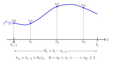
This source-controlled course schematic was re-authored from the mathematical layout of Biegler (2010), Figure 10.1; it is not a reproduction of the textbook artwork.

The collocation method can be developed by solving the differential equation ( $dz/dt$ ) at specific time points. For example, Figure 10.1 shows the state variable approximation for a single finite element:

\begin{align} z^k(t) = \alpha_0 + \alpha_1t + ... + \alpha_kt^k \end{align}

(9)

where $\alpha_n$ are constants in the power series. This profile can also be represented as a Lagrange interpolation polynomial. Choosing $K+1$ interpolation points within element $i$ , the state can be represented as:

\begin{align} & t = t_{i-1} + h_i\tau , \\ & z^k(t) = \sum_{j=0}^K \ell_j(\tau)z_{ij} , \\ & \text{for } t \in [t_{i-1},t_i] \text{ and } \tau \in [0,1] , \\ & \text{where } \ell_j(\tau) = \prod_{k=0,\neq j}^K \frac{(\tau-\tau_k)}{(\tau_j-\tau_k)} \\ & \tau_0=0 \\ & \tau_j<\tau_{j+1}, \\ & j=0,...,K-1 , \\ & \text{and } h_i \text{ is the length of element } i. \\ \end{align}

(10)

The key property of this polynomial is that $z^K(t_{ij})=z_{ij}$ where $t_{ij}=t_{i-1} + \tau_j h_i$ .

We can do the same thing for the time derivative of the state (Lagrange polynomial with K interpolation points):

\begin{align} z^K(t) = z_{i-1} + h_i \sum_{j=1}^K \Omega_j(\tau) \dot{z}_{ij} , \end{align}

(11)

where $z_{i-1}$ represents the differential state at the beginning of element $i$ , $\dot{z}_{ij}$ is the time derivative, and $\Omega_j(\tau)$ is a $K^{th}$ order polynomial that satisfies:

\begin{align} \Omega_j(\tau)=\int_0^{\tau}\ell_j(\tau')d\tau', \text{ }t \in [t_{i-1},t_i], \text{ }\tau \in [0,1]. \end{align}

(12)

This is the implicit Runge--Kutta (IRK) representation with $n_s=K$ , $c_k=\tau_k$ , $a_{kj}=\Omega_j(\tau_k)$ , and $b_j=\Omega_j(1)$ . The basis functions are determined by the chosen collocation nodes.

Collocation equations can be found by substituting the polynomial into the differential equation ( $dz/dt$ ). The algebraic equations must hold at each interpolation point $\tau_j$ . The collocation equations for the Lagrange polynomial are:

\begin{align} \sum_{j=0}^K z_{ij} \frac{d\ell_j(\tau_k)}{d\tau}=h_i f(z_{ik},t_{ik}), \text{ } k=1,...,K. \end{align}

(13)

Collocation with Orthogonal Polynomials¶

With the interpolation points $\tau_k$ known, then the collocation equations become algebraic. Now $\tau_k$ must be determined such that the approximation is most accurate. Representing the solution as an integral:

\begin{align} z(t_i) = z(t_{i-1}) + \int_{t_{i-1}}^{t_i} f(z(t),t)dt , \end{align}

(14)

the numerical solution is the quadrature formula:

\begin{align} & z(t_i) = z(t_{i-1}) + \sum_{j=1}^K \omega_j h_i f(z(t_{ij}), t_{ij}), & t_{ij} = t_{i-1} + h_i \tau_j \end{align}

(15)

Theorem 10.1: The quadrature formula above is exact when $f(z(t),t)$ is a polynomial in $t$ of order $2K$ —that is, degree at most $2K-1$ in Biegler’s terminology—and $\tau_j$ are the roots of a $K$ th-degree polynomial $P_K(\tau)$ with the property:
$\begin{align} & \int_0^1 P_j(\tau) P_{j'}(\tau)d\tau = 0, & j=0,...,K-1, & \text{ } j'=1,...,K, & \text{for indices } j \neq j'. \end{align}$
(16)

This theorem justifies choosing the collocation points ( $\tau_j$ ) as the roots of $P_K(\tau)$ . $P_K(\tau)$ is the shifted Gauss-Legendre polynomial that has the orthogonality property as shown by the result of the theorem. This polynomial can be broadly classified as a Gauss-Jacobi polynomial. See Section 10.2.2 of Biegler for more information.

Using the roots of the Gauss-Jacobi polynomials as collocation points leads to the following results:

Gauss-Legendre collocation leads to truncation error of $O(h^{2k})$
Gauss-Radau collocation leads to truncation error of $O(h^{2k-1})$

Generally, Gauss-Legendre and Radau collocation are compatible with NLP formulations.

Applications to Runge-Kutta¶

When the Runge-Kutta basis is applied, the collocation method is seen to be an IRK method, leading to the following properties (established in Biegler Section 9.2):

Gauss--Legendre and Radau collocation formulas are A-stable and algebraically stable. For the linear test equation, A-stability removes a step-size restriction imposed solely by absolute stability when the eigenvalue lies in the left half-plane. Accuracy and nonlinear convergence can still require smaller elements; A-stability is not permission to choose $h_i$ arbitrarily.
Radau collocation has stiff decay. Therefore, if your problem is stiff, try Radau collocation first.
Gauss-Legendre and Radau collocation methods have high-order error. (Here, order refers to $z_i$ .)

A Final Key Note¶

Continuity is enforced in states across finite element boundaries, NOT controls or algebraic variables.