Numeric Integration for DAEs - Optimization for Decision Science

Prepared by: Prof. Alexander Dowling, Myia Dickens (mdicken2@nd.edu,2023)

This notebook is the computational companion to Lectures 5--7. It connects error and stability experiments for ODE integrators to index-1 DAE integration, then prepares for direct collocation in Pyomo.dae.

import sys

if "google.colab" in sys.modules:
    !wget "https://raw.githubusercontent.com/ndcbe/optimization/main/notebooks/helper.py"
    # Do not need casadi for this notebook
    #!pip install casadi
    import helper

    helper.easy_install()
else:
    sys.path.insert(0, "../")
    import helper
helper.set_plotting_style()


import numpy as np
import scipy.optimize as opt
import matplotlib.pyplot as plt

Single-Step Runge-Kutta Methods¶

Chapter 9 in Biegler (2010)
Chapter 17 in McClarren (2018)

General Form: Index 0 DAE¶

Consider the ODE system:

\dot{z} = f(t,z), \quad z(t_0) = z_0

(1)

where $z(t)$ are the differential variables and $f(t,z)$ is a (nonlinear) continuous function.

The general Runge-Kutta formula is:

\begin{align} z_{i+1} &= z_{i} + h_i \sum_{k=1}^{n_s} b_k f(t_i + c_k h_i, \hat{z}_k) \\ \hat{z}_k &= z_i + h_i \sum_{j=1}^{n_{rk}} a_{k,j} f(t_i + c_j h_i, \hat{z}_j), \quad k=1,...,n_s \end{align}

(2)

where

$z_i$ are the differential variables at the start of step $i$ (time $t_i$ )
$z_{i+1}$ are the differential variables at the end of step $i$ (time $t_{i+1}$ )
$\hat{z}_k$ are differential variables for intermediate stage $k$
$h_i$ is the size for step $i$ such that $t_{i+1} = t_i + h_i$
$n_s$ is the number of stages
$n_{rk}$ is the number of $f(\cdot)$ evaluations to calculate intermediate $k$
$a_{k,j}$ are coefficients, together known as the Runge-Kutta matrix
$b_k$ are coefficients, known as the weights
$c_k$ are coefficients, known as the nodes

$h_i$ is selected based on error tolerances

The choice for $A$ , $b$ and $c$ selects the specific method in the Runge-Kutta family. These coefficients are often specified in a Butcher block (or Butcher tableau).

A Runge-Kutta method is called consistent if:

\sum_{k=1}^{n_s} b_k = 1 \quad \mathrm{and} \quad \sum_{j=1}^{n_s} a_{k,j} = c_k

(3)

Explicit (Forward) Euler¶

Consider one of the simplest Runge-Kutta methods:

z_{i+1} = z_{i} + h_i~f(t_i, z_i)

(4)

What are $A$ , $b$ and $c$ in the general formula?

$n_s = 1$ . This is only a single stage. Thus we only need to determine $c_1$ , $b_1$ , and $n_{r1}$

Moreover, $\hat{z}_1 = z_i$ because $f(\cdot)$ is only evaluated at $t_i$ and $z_i$ . This implies:

$n_{r1} = 0$
$c_1 = 0$
$b_1 = 1$
$A$ is empty because $n_{r1} = 0$

The implementation is very straightforward (see below). We can calculate $z_{i+1}$ with a single line!

def create_steps(tstart, tend, dt):
    n = int(np.ceil((tend - tstart) / dt))
    return dt * np.ones(n)


def explicit_euler(f, h, z0):
    """
    Arguments:
        f: function that returns rhs of ODE
        h: list of step sizes
        z0: initial conditions

    Returns:
        t: list of time steps. t[0] is 0.0 by default
        z: list of differential variable values
    """

    # Number of timesteps
    nT = len(h) + 1

    t = np.zeros(nT)

    # Number of states
    nZ = len(z0)
    Z = np.zeros((nT, nZ))

    # Copy initial states
    Z[0, :] = z0

    for i in range(1, nT):

        i_ = i - 1

        # Advance time
        t[i] = t[i_] + h[i_]

        # Explicit Euler formula
        Z[i, :] = Z[i_, :] + h[i_] * f(t[i_], Z[i_, :])

    return t, Z

Implicit (Backward) Euler¶

Consider another simple Runge-Kutta method:

z_{i+1} = z_{i} + h_i~f(t_{i+1}, z_{i+1})

(5)

What are $A$ , $b$ and $c$ to express using the general formula?

$n_s = 1$ . This is only a single stage. Moreover, $\hat{z}_1 = z_{i+1}$ because $f(\cdot)$ is evaluated at $t_{i+1}$ and $z_{i+1}$ . This implies:

$b_1 = 1$
$c_1 = 1$

Moreover, $z_{i+1} = z_{i} + h_i~f(t_{i+1}, z_{i+1})$ implies $\hat{z}_1 = z_i + h_i f(t_{i+1}, \hat{z}_1)$ . Thus:

$a_{1,1} = 1$

Notice that the formula for $z_{i+1}$ is implicit. We need to solve a (nonlinear) system of equations to calculate the step.

def implicit_euler(f, h, z0):
    """
    Arguments:
        f: function that returns rhs of ODE
        h: list of step sizes
        z0: initial conditions

    Returns:
        t: list of time steps. t[0] is 0.0 by default
        z: list of differential variable values
    """

    # Number of timesteps
    nT = len(h) + 1

    t = np.zeros(nT)

    # Number of states
    nZ = len(z0)
    Z = np.zeros((nT, nZ))

    # Copy initial states
    Z[0, :] = z0

    for i in range(1, nT):

        i_ = i - 1

        # Advance time
        t[i] = t[i_] + h[i_]

        ## Implicit Runge-Kutta formula.
        ## Need to solve nonlinear system of equations.

        # Use Explicit Euler to calculate initial guess
        Z[i, :] = Z[i_, :] + h[i_] * f(t[i_], Z[i_, :])

        # Solve nonlinear equation
        implicit = lambda z: Z[i_, :] + h[i_] * f(t[i], z) - z
        Z[i, :] = opt.fsolve(implicit, Z[i, :])

    return t, Z

Key Differences¶

Explicit Methods	Implicit Methods
+ Easy to Program	- Requires converging system of nonlinear equations
- Stability regions are often bounded, so stability can restrict $h_i$	+ Stability regions are often larger or unbounded, but still depend on the method and problem

Comparison¶

Let’s test this on a simple problem:

\dot{z}(t) = -\lambda z(t), \qquad z_0 = 1.

(6)

The solution to this problem is

z(t) = e^{-\lambda t}.

(7)

For simplicity, let’s numerically analyze $\lambda = 1$ .

$Forward and backward Euler on \dot z = -z at h=1.0 and h=2.5: below the bound h<2/\lambda both methods decay; above it forward Euler oscillates and grows while backward Euler does not.$

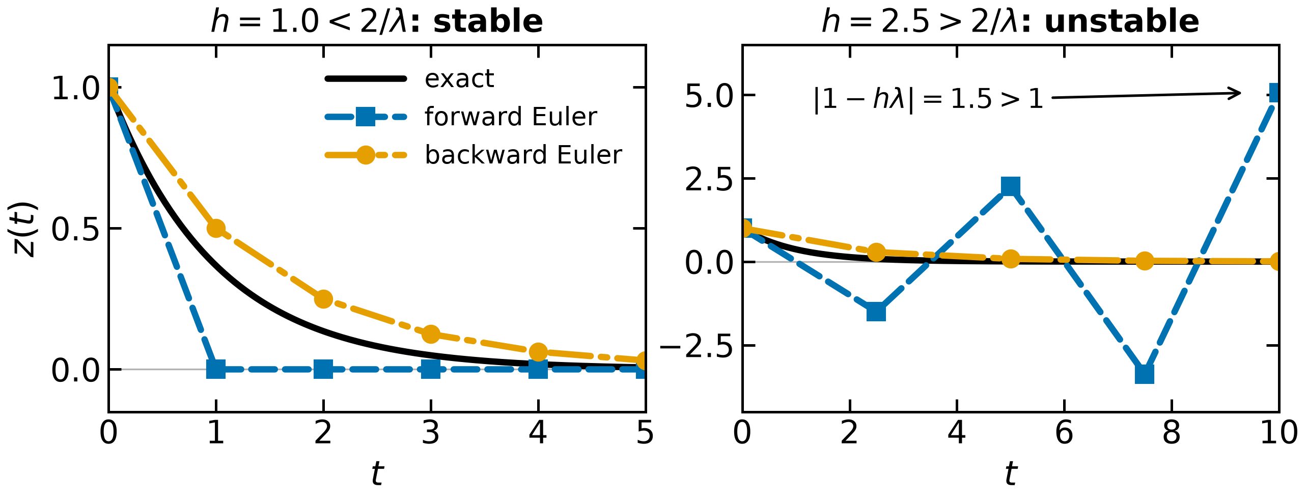
The stability contrast in one picture, rendered from figures/plots/euler-stability.py. This is the same image printed in the course pack, so the handout and the website cannot drift apart.

Run the two cells below to reproduce each panel yourself and to change dt.

rhs = lambda t, z: -z
sln = lambda t: np.exp(-t)

dt = 1.0
h = create_steps(0.0, 5.0, dt)

z0 = [1]

te, Ze = explicit_euler(rhs, h, z0)
ti, Zi = implicit_euler(rhs, h, z0)

plt.figure()

# Use 101 points for exact to make it smooth
texact = np.linspace(0.0, np.sum(h), 101)

# Plot solutions
plt.plot(texact, sln(texact), label="Exact Solution")
plt.plot(te, Ze, marker="s", label="Forward Euler")
plt.plot(ti, Zi, marker="o", label="Backward Euler")
plt.xlabel("t")
plt.ylabel("z")
plt.legend()
plt.title("Solution with h = " + str(dt))
plt.show()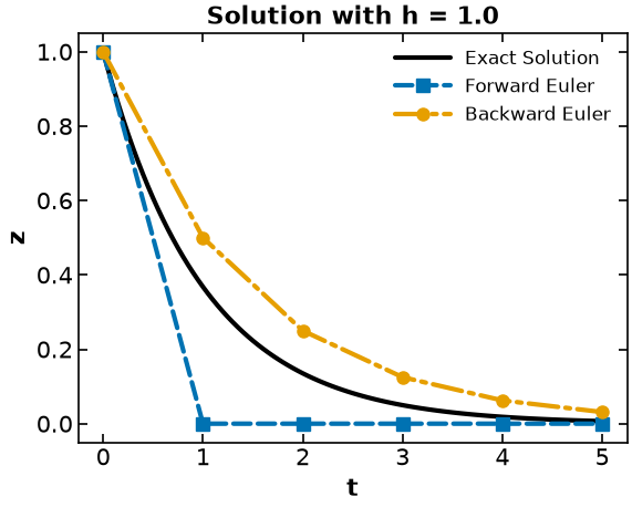

Stability¶

Keeping $\lambda = 1$ , are there any limits on step size?

dt = 2.5
h = create_steps(0.0, 10.0, dt)

z0 = [1]

te, Ze = explicit_euler(rhs, h, z0)
ti, Zi = implicit_euler(rhs, h, z0)

plt.figure()

# Use 101 points for exact to make it smooth
texact = np.linspace(0.0, np.sum(h), 101)

# Plot solutions
plt.plot(texact, sln(texact), label="Exact Solution")
plt.plot(te, Ze, marker="s", label="Forward Euler")
plt.plot(ti, Zi, marker="o", label="Backward Euler")
plt.xlabel("t")
plt.ylabel("z")
plt.legend()
plt.title("Solution with h = " + str(dt))
plt.show()

/var/folders/3w/vr4xmyqs451dg23xk88pqcg00000gq/T/ipykernel_47280/1577139293.py:40: RuntimeWarning: The iteration is not making good progress, as measured by the 
 improvement from the last ten iterations.
  Z[i, :] = opt.fsolve(implicit, Z[i, :])

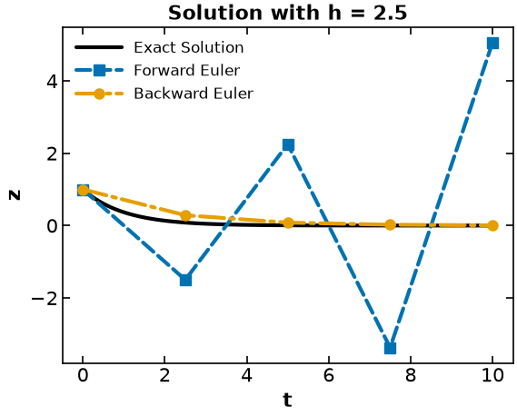
Key observation: forward (explicit) Euler becomes unstable with large steps whereas backward (implicit) Euler is stable.

The Lecture 6 handout derives the growth factors and then generalizes them to absolute-stability regions.

Key results (for this specific test problem):

Forward Euler is stable for this problem when $h\lambda \leq 2$ and non-oscillatory when $h\lambda \leq 1$ .
Backward Euler is stable and non-oscillatory for every $h > 0$ when $\lambda > 0$ .
Crank--Nicolson is stable for every $h > 0$ , but oscillates when $h\lambda > 2$ .
Similar analysis and concepts extend to Runge-Kutta methods.

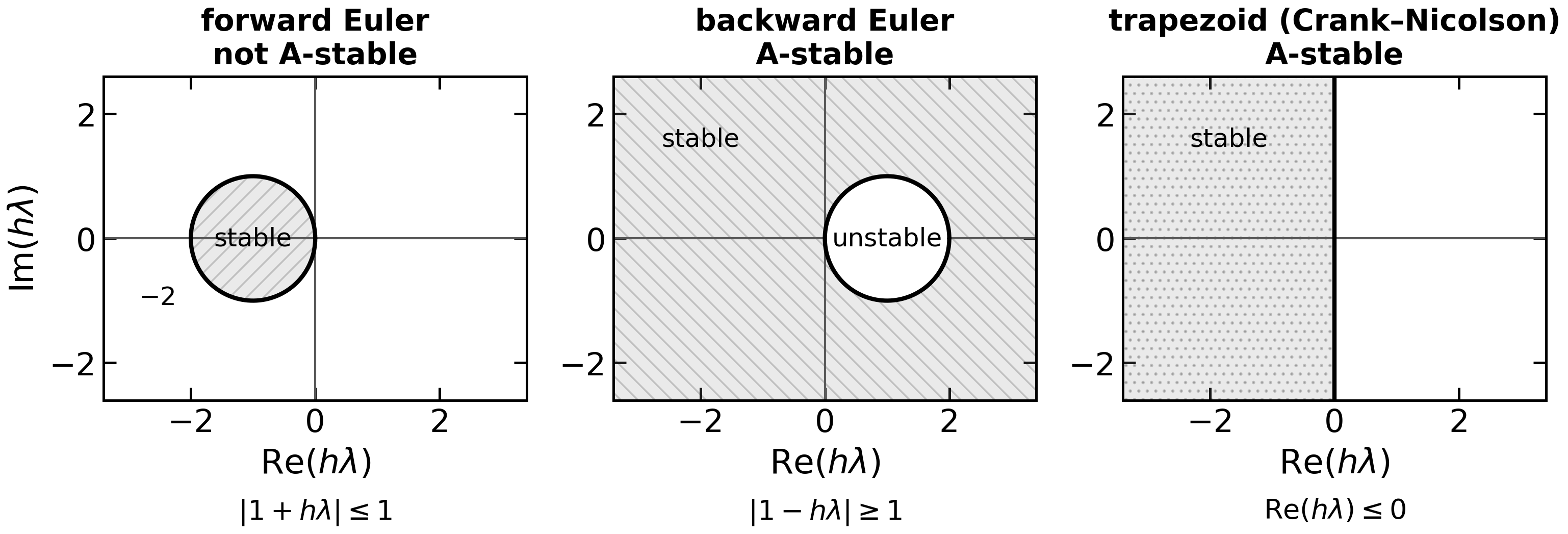
Regions of absolute stability in the complex h-lambda plane: forward Euler is a bounded disc, backward Euler is the exterior of a disc, Crank-Nicolson is exactly the left half-plane.

Why the step-size limit exists, in one picture. Rendered from figures/plots/stability-regions.py; the same image printed in the course pack.

The shaded set is where the method does not amplify. A method is A-stable when that set covers the entire left half-plane (Ascher & Petzold, p. 56). Forward Euler’s region is bounded, so it never can be -- hence $h < 2/\lambda$ . Backward Euler and Crank-Nicolson both are.

Error Analysis¶

How does our choice in step size $h$ impact the error of these numerical techniques?

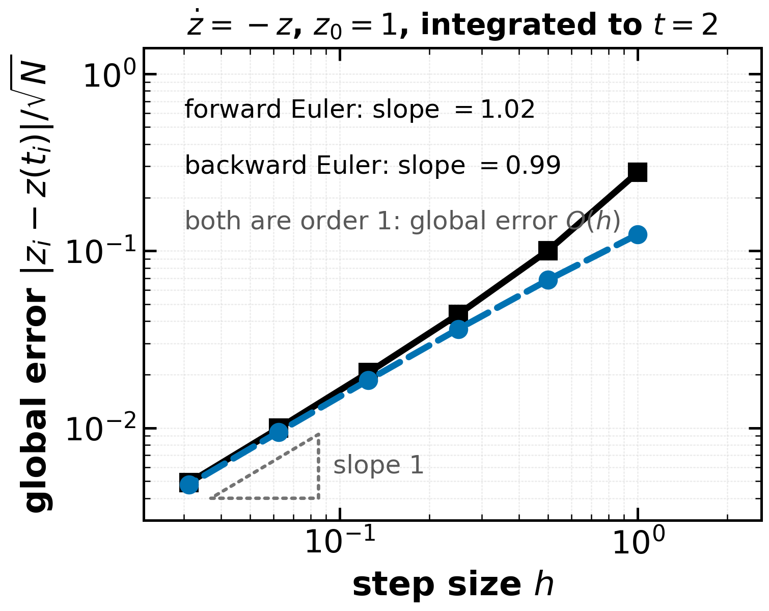
$Global error vs step size for forward and backward Euler on \dot z=-z, log-log axes; both slopes are 1.$

The order of accuracy, measured rather than asserted. Rendered from figures/plots/euler-error-order.py. This is the same image printed in the course pack, so the handout and the website cannot drift apart.

Both slopes are 1, not 2. Forward and backward Euler each commit $O(h^2)$ on a single step, but a fixed interval takes $N \propto 1/h$ steps, so the global error is $O(h)$ -- one order is paid away to the step count. Read the slope, not the per-step order.

Run the cell below to reproduce it yourself and to change the step list.

Delta_t = np.array([1.0, 0.5, 0.25, 0.125, 0.0625, 0.0625 / 2])
t_final = 2
error_forward = np.zeros(Delta_t.size)
error_backward = np.zeros(Delta_t.size)

for i in range(0, len(Delta_t)):

    # create steps
    h = create_steps(0.0, t_final, Delta_t[i])

    # solve
    t, ze = explicit_euler(rhs, h, z0)
    t, zi = implicit_euler(rhs, h, z0)
    zsln = np.exp(-t)

    n = len(t) - 1

    # Calculate error
    error_forward[i] = np.linalg.norm(ze[:, 0] - zsln) / np.sqrt(n)
    error_backward[i] = np.linalg.norm(zi[:, 0] - zsln) / np.sqrt(n)


plt.loglog(Delta_t, error_forward, "s-", color="red", label="Forward Euler")
plt.loglog(Delta_t, error_backward, "o-", color="blue", label="Backward Euler")

# slope = (np.log(error[-1]) - np.log(error[-2]))/(np.log(Delta_t[-1])- np.log(Delta_t[-2]))
# plt.title("Slope of Error is " + str(slope))
plt.xlabel("Step Size (h)")
plt.ylabel("Norm of Error")
plt.show()

# Calculate slope
calc_slope = lambda error: (np.log(error[-1]) - np.log(error[-2])) / (
    np.log(Delta_t[-1]) - np.log(Delta_t[-2])
)

print("Slope for Forward Euler: " + str(calc_slope(error_forward)))
print("Slope for Backward Euler: " + str(calc_slope(error_backward)))

/var/folders/3w/vr4xmyqs451dg23xk88pqcg00000gq/T/ipykernel_47280/1577139293.py:40: RuntimeWarning: The iteration is not making good progress, as measured by the 
 improvement from the last ten iterations.
  Z[i, :] = opt.fsolve(implicit, Z[i, :])

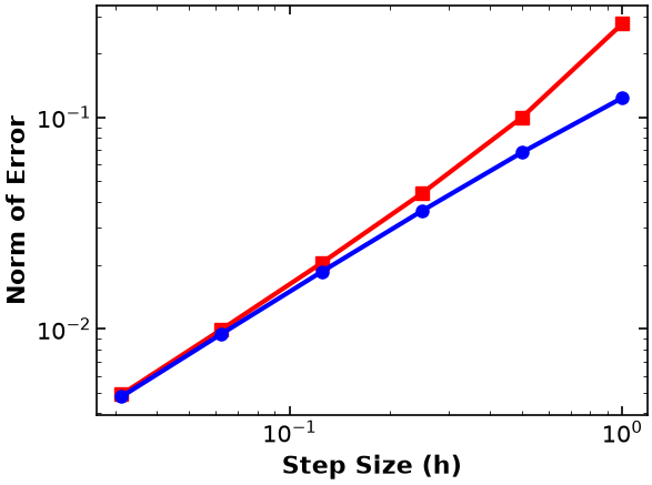
Slope for Forward Euler: 1.0220608473216777
Slope for Backward Euler: 0.9874086317220971

Both Euler methods are first order in $\Delta t$ : halving $\Delta t$ approximately halves the global error. Here we measure the error with the root-mean-square norm

\mathrm{Error} = \frac{1}{\sqrt{N}}\sqrt{\sum_{n=1}^{N} \left(y^n_\mathrm{approx} - y^n_\mathrm{exact}\right)^2},

(8)

where $N$ is the number of steps the ODE is solved over.

Key Results:

Implicit and Explicit Euler have $O(h^2)$ local error and $O(h)$ global error.

Extending Numeric Integration to Index-1 DAEs¶

Consider semi-explicit DAEs:

\begin{aligned} \dot{z} = f(t,z,y), \quad g(z,y) = 0, \quad z(t_0) = z_0 \end{aligned}

(9)

Runge-Kutta methods are easy to extend.

\begin{aligned} z_{i+1} &= z_{i} + h_i \sum_{k=1}^{n_s} b_k f(t_i + c_k h_i, \hat{z}_k, \hat{y}_k) \\ \hat{z}_k &= z_i + h_i \sum_{j=1}^{n_{rk}} a_{k,j} f(t_i + c_j h_i, \hat{z}_j, \hat{y}_j), \quad k=1,...,n_s \\ 0 &= g(\hat{z}_k, \hat{y}_k), \quad k=1,...,n_s \end{aligned}

(10)

Backward differentiation formulas (BDFs) also extend to index-1 DAEs. Backward Euler is the one-step, first-order member of this family.

\begin{aligned} z_{i+1} &= \sum_{j=1}^{n_s} \alpha_j z_{i-j+1} + \beta_0 hf(z_{i+1},y_{i+1})\\ 0 &= g(z_{i+1},y_{i+1}) \end{aligned}

(11)

At each BDF step, solve the coupled equations for $(z_{i+1},y_{i+1})$ with Newton’s method. Using the conventional row-by-variable Jacobian and the residual $z_{i+1}-\sum_j \alpha_j z_{i-j+1}-\beta_0 h f(z_{i+1},y_{i+1})=0$ , the Jacobian is:

\begin{aligned} J(z_{i+1},y_{i+1}) &= \begin{bmatrix} I - h\beta_0\frac{\partial f}{\partial z} & -h\beta_0\frac{\partial f}{\partial y} \\ \frac{\partial g}{\partial z} & \frac{\partial g}{\partial y} \end{bmatrix} \end{aligned}

(12)

This follows Biegler (2010), equations (9.18)--(9.19), pp. 259--260, with two corrections made explicit: derivatives here use the course’s row-by-variable convention, and the upper-right block has a minus sign when the first residual is written in the form above. The printed equation (9.19) combines the opposite sign in that block with $I-h\beta_0 f_z$ ; direct differentiation shows those signs cannot belong to the same residual, and the published errata do not list the issue.

Key Results. For an index-1 DAE, implicit RK and BDF extensions generally retain ODE-like order and stability properties, subject to method-specific order-reduction and stability limitations.

Discussion: Why are implicit methods usually preferred for index-1 DAE systems?

Backward Euler transcription of an ODE-constrained optimization problem¶

Reference: Bynum, Hackebeil, Hart, Laird, Nicholson, Siirola, Watson & Woodruff, Pyomo — Optimization Modeling in Python, 3rd ed., Springer (2021), §12.1, p. 181, equations (12.1)–(12.6). (Earlier versions of this notebook cited “Hart, 2010”, which is the 1st edition — a different book with different pagination.)

The example below is an ODE model with a path inequality, not a DAE. It shows how backward Euler exposes time-indexed states, controls, and constraints to an optimization solver.

Consider the following optimal control problem

\begin{align} \min_{u(t)} \quad & x_3(t_f) \\ \mathrm{s.t.} \quad & \dot{x}_1 = x_2 \\ & \dot{x}_2 = -x_2 + u(t) \\ & \dot{x}_3 = x_1^2 + x_2^2 + 0.005 \cdot u^2 \\ & x_2 - 8 \cdot (t-0.5)^2 + 0.5 \leq 0 \\ & x_1(0) = 0, x_2(0) = -1, x_3(0) = 0, t_f = 1 \end{align}

(13)

Discussion: What variable is the problem attempting to minimize? What variable is being optimized? What types of equations are there?

import pyomo.environ as pyo
import pyomo.dae as dae

No Pyomo units in this model, and two separate reasons why.

The dynamic optimization notebooks in this section declare units= on every Var and Param and check them with assert_units_consistent before discretizing -- see Units in Pyomo.dae Models. This model is an honest exception on both counts.

The states are abstract. $x_1$ , $x_2$ , $x_3$ come from the Pyomo book’s §12.1 test problem. They have no physical referent, so any units we assigned would be invented. Inventing units is worse than omitting them: it produces a check that looks meaningful and is not.

The path constraint indexes time directly. Look at the rule:

def _con(m, t):
    return m.x2[t] - 8 * (t - 0.5) ** 2 + 0.5 <= 0

That t is a bare Python float -- the raw ContinuousSet index that Pyomo passed into the rule. It is not a Pyomo object and it carries no units, so there is nothing to attach units to. This is the cleanest illustration in the course of Pyomo issue #1790 (add units support to ContinuousSet/Pyomo.dae, still open): a ContinuousSet cannot hold units, which is also why a units-correct Pyomo.dae model passes assert_units_consistent before discretization and fails after it.

When a model is physical and needs a time-dependent reference trajectory, the workaround is to have the helper return a bare number and multiply by the intended units at the call site. Hot Air Balloon Dynamic Control does exactly that.

def create_dynamic_optimization_model():

    # Create model
    m = pyo.ConcreteModel()

    # Declare time set
    m.tf = pyo.Param(initialize=1)  # final time
    m.t = dae.ContinuousSet(bounds=(0, m.tf))

    # Declare constraint and input variables
    m.u = pyo.Var(m.t, initialize=0)
    m.x1 = pyo.Var(m.t)
    m.x2 = pyo.Var(m.t)
    m.x3 = pyo.Var(m.t)

    # Declare differential variables
    m.dx1 = dae.DerivativeVar(m.x1, wrt=m.t)
    m.dx2 = dae.DerivativeVar(m.x2, wrt=m.t)
    m.dx3 = dae.DerivativeVar(m.x3)

    # Declare differential equations
    @m.Constraint(m.t)
    def x1dotcon(m, t):
        if t == m.t.first():
            return pyo.Constraint.Skip
        return m.dx1[t] == m.x2[t]

    @m.Constraint(m.t)
    def x2dotcon(m, t):
        if t == m.t.first():
            return pyo.Constraint.Skip
        return m.dx2[t] == -m.x2[t] + m.u[t]

    @m.Constraint(m.t)
    def x3dotcon(m, t):
        if t == m.t.first():
            return pyo.Constraint.Skip
        return m.dx3[t] == m.x1[t] ** 2 + m.x2[t] ** 2 + 0.005 * m.u[t] ** 2

    # Declare inequality constraints
    @m.Constraint(m.t)
    def con(m, t):
        return m.x2[t] - 8 * (t - 0.5) ** 2 + 0.5 <= 0

    # Declare the initial conditions
    @m.Constraint()
    def init_x1(m):
        return m.x1[0] == 0

    @m.Constraint()
    def init_x2(m):
        return m.x2[0] == -1

    @m.Constraint()
    def init_x3(m):
        return m.x3[0] == 0

    # Declare Objective function
    m.obj = pyo.Objective(expr=m.x3[m.tf])

    return m


# Discretize and solve using backward Euler
def solve_with_backward_euler(m):
    """
    Arguments:
      m: Pyomo.DAE dynamic optimization model
    New Elements:
      nfe = number for finite elements - specifies the number of discretization points to be used
    Purpose:
      Discretizes the ODE constraints with backward Euler and solves the NLP
    """

    discretizer = pyo.TransformationFactory("dae.finite_difference")
    discretizer.apply_to(m, nfe=20, wrt=m.t, scheme="BACKWARD")

    solver = pyo.SolverFactory("ipopt")
    results = solver.solve(m, tee=True)
    assert pyo.check_optimal_termination(results), (
        f"Solve failed: status={results.solver.status}, "
        f"termination={results.solver.termination_condition}"
    )


# Plot the results
def plotter(subplot, x, *y, **kwds):
    plt.subplot(subplot)
    # Color AND linestyle, so the figure survives a black-and-white printout.
    linestyles = ["-", "--", "-.", ":"]
    for i, _y in enumerate(y):
        plt.plot(
            list(x),
            [pyo.value(_y[t]) for t in x],
            color="brgcmk"[i % 6],
            linestyle=linestyles[i % 4],
        )
        if kwds.get("points", False):
            plt.plot(list(x), [pyo.value(_y[t]) for t in x], "o")
    plt.title(kwds.get("title", ""), fontsize=16, fontweight="bold")
    plt.tick_params(direction="in", labelsize=15)
    plt.legend(tuple(_y.name for _y in y))
    plt.xlabel(x.name, fontsize=16, fontweight="bold")


def plot_results(m):
    plotter(121, m.t, m.x1, m.x2, title="Differential Variables")
    plotter(122, m.t, m.u, title="Control Variable", points=True)
    plt.show()


# Create model
model = create_dynamic_optimization_model()

# Solve the discretized dynamic optimization problem
results = solve_with_backward_euler(model)

Ipopt 3.14.19: 

******************************************************************************
This program contains Ipopt, a library for large-scale nonlinear optimization.
 Ipopt is released as open source code under the Eclipse Public License (EPL).
         For more information visit https://github.com/coin-or/Ipopt
******************************************************************************

This is Ipopt version 3.14.19, running with linear solver MUMPS 5.8.2.

Number of nonzeros in equality constraint Jacobian...:      363
Number of nonzeros in inequality constraint Jacobian.:       21
Number of nonzeros in Lagrangian Hessian.............:       60

Total number of variables............................:      143
                     variables with only lower bounds:        0
                variables with lower and upper bounds:        0
                     variables with only upper bounds:        0
Total number of equality constraints.................:      123
Total number of inequality constraints...............:       21
        inequality constraints with only lower bounds:        0
   inequality constraints with lower and upper bounds:        0
        inequality constraints with only upper bounds:       21

iter    objective    inf_pr   inf_du lg(mu)  ||d||  lg(rg) alpha_du alpha_pr  ls
   0  0.0000000e+00 1.00e+00 2.82e-01  -1.0 0.00e+00    -  0.00e+00 0.00e+00   0
   1  0.0000000e+00 1.24e+00 6.10e-01  -1.0 1.57e+01    -  6.19e-01 1.00e+00f  1
   2  3.3913637e-01 2.47e-01 1.00e-06  -1.0 5.83e+00    -  1.00e+00 1.00e+00f  1
   3  3.3096072e-01 1.37e-02 2.00e-07  -1.7 1.05e+00    -  1.00e+00 1.00e+00h  1
   4  1.5256107e-01 5.24e-02 1.50e-09  -3.8 9.83e-01    -  1.00e+00 1.00e+00h  1
   5  1.4973078e-01 9.43e-03 1.50e-09  -3.8 6.08e-01    -  1.00e+00 1.00e+00h  1
   6  1.4923815e-01 1.41e-03 1.50e-09  -3.8 3.46e-01    -  1.00e+00 1.00e+00h  1
   7  1.4795692e-01 3.28e-04 4.99e-05  -5.7 1.84e-01    -  1.00e+00 9.88e-01h  1
   8  1.4798373e-01 1.22e-05 1.84e-11  -5.7 3.85e-02    -  1.00e+00 1.00e+00h  1
   9  1.4796950e-01 7.16e-08 2.51e-14  -8.6 2.69e-03    -  1.00e+00 1.00e+00h  1

iter    objective    inf_pr   inf_du lg(mu)  ||d||  lg(rg) alpha_du alpha_pr  ls
  10  1.4796952e-01 6.90e-13 2.51e-14  -8.6 1.15e-05    -  1.00e+00 1.00e+00h  1

Number of Iterations....: 10

                                   (scaled)                 (unscaled)
Objective...............:   1.4796951825372692e-01    1.4796951825372692e-01
Dual infeasibility......:   2.5063284780912909e-14    2.5063284780912909e-14
Constraint violation....:   6.9008687653138168e-13    6.9008687653138168e-13
Variable bound violation:   0.0000000000000000e+00    0.0000000000000000e+00
Complementarity.........:   2.5060342008003911e-09    2.5060342008003911e-09
Overall NLP error.......:   2.5060342008003911e-09    2.5060342008003911e-09


Number of objective function evaluations             = 11
Number of objective gradient evaluations             = 11
Number of equality constraint evaluations            = 11
Number of inequality constraint evaluations          = 11
Number of equality constraint Jacobian evaluations   = 11
Number of inequality constraint Jacobian evaluations = 11
Number of Lagrangian Hessian evaluations             = 10
Total seconds in IPOPT                               = 0.254

EXIT: Optimal Solution Found.

# Plot solution
plot_results(model)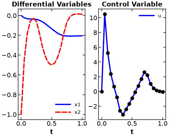

Stiff chemical-reaction example¶

Consider consecutive first-order reactions $A \rightarrow B \rightarrow C$ with $k_1=1000$ and $k_2=1$ :

\dot{c} = \begin{bmatrix} -k_1 & 0 & 0 \\ k_1 & -k_2 & 0 \\ 0 & k_2 & 0\end{bmatrix} c, \qquad c(0) = [1, 0, 0]^T .

(14)

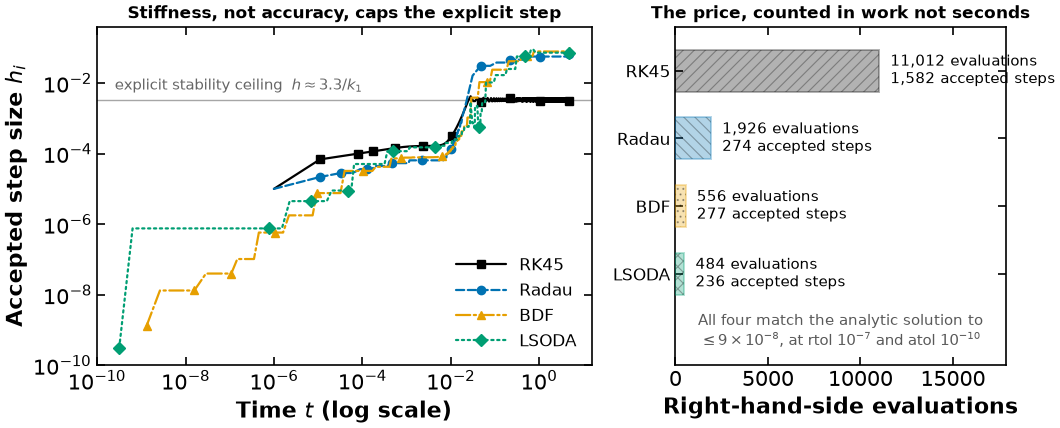
The Jacobian eigenvalues are $-k_1$ , $-k_2$ and 0, so the stiffness ratio is $k_1/k_2 = 1000$ : $A$ disappears in about $1/k_1 = 1$ ms while $B$ is still converting a thousand times more slowly. We compare one explicit adaptive method (RK45) with three methods designed for, or able to detect, stiffness (Radau, BDF, LSODA).

Use the same tolerances for every method, and compare solver work through accepted steps and right-hand-side evaluations rather than wall time, which varies substantially across computers and Colab sessions.

# ---------- MODEL ----------------------------------------------------------
# Consecutive first-order reactions  A --k1--> B --k2--> C  with k1 = 1000 and
# k2 = 1. The Jacobian's eigenvalues are -k1, -k2 and 0, so the stiffness ratio
# is k1/k2 = 1000: A disappears on a timescale of 1/k1 = 1 ms while B is still
# converting on a timescale of 1/k2 = 1 s.
#
# The system is LINEAR, so the Jacobian is constant and exact. That is
# deliberate: Radau and BDF are handed the analytic Jacobian, which removes
# "how good is the finite-difference Jacobian" as an explanation for the work
# counts below. It also gives an analytic solution to measure error against.
from scipy.integrate import solve_ivp

k1, k2 = 1000.0, 1.0

reaction_jacobian = np.array([[-k1, 0.0, 0.0],
                              [k1, -k2, 0.0],
                              [0.0, k2, 0.0]])


def reaction_rhs(t, concentration):
    """d[A, B, C]/dt for the consecutive first-order reactions."""
    return reaction_jacobian @ concentration


def reaction_exact(t):
    """Analytic solution from [A, B, C](0) = [1, 0, 0]; rows are A, B, C.

    A = e^{-k1 t},  B = k1/(k1 - k2) (e^{-k2 t} - e^{-k1 t}),  C = 1 - A - B.
    Used as the accuracy reference, so "cheap" cannot be confused with "loose".
    """
    t = np.asarray(t, dtype=float)
    a = np.exp(-k1 * t)
    b = k1 / (k1 - k2) * (np.exp(-k2 * t) - np.exp(-k1 * t))
    return np.vstack([a, b, 1.0 - a - b])

# ---------- SOLVE + EXTRACT ------------------------------------------------
# Everything below this cell reads `results` and nothing else. The archive
# figures/results/stiff-solver-comparison.json stores the DATA -- the accepted
# step sequence, the work counters and the measured error for each method -- so
# the figure can be restyled later without re-integrating. See figures/README.md
# and figures/render_from_notebook.py for the cell contract.
#
# ⚠ EVERY METHOD GETS THE SAME TOLERANCES. Comparing work at different
# tolerances measures nothing, so rtol/atol are fixed here and the achieved
# error is measured afterwards to confirm the four answers really are
# comparable.
#
# ⚠ WORK, NOT WALL TIME. Prof. Dowling's standing instruction for this
# comparison: count right-hand-side evaluations and accepted steps, which are
# properties of the method and the problem, not of the laptop or the Colab VM
# the notebook happens to run on.

t_final = 5.0
rtol, atol = 1e-7, 1e-10
transient_end = 0.5   # after this, A is gone and only the slow B -> C remains

# Dormand-Prince's real-axis absolute-stability boundary is h|lambda| ~ 3.3.
# With lambda = -k1 that caps the explicit step at ~3.3/k1 no matter how smooth
# the solution has become -- which is the whole argument of this section.
explicit_step_ceiling = 3.3 / k1

method_kind = {"RK45": "explicit", "Radau": "implicit",
               "BDF": "implicit", "LSODA": "switching"}

t_check = np.linspace(0.0, t_final, 2001)
exact_check = reaction_exact(t_check)

methods_out = []
solutions = {}   # kept for the concentration-profile diagnostic below
for method in ("RK45", "Radau", "BDF", "LSODA"):
    options = {"jac": reaction_jacobian} if method in ("Radau", "BDF") else {}
    solution = solve_ivp(
        reaction_rhs, (0.0, t_final), [1.0, 0.0, 0.0], method=method,
        rtol=rtol, atol=atol, dense_output=True, **options
    )

    solutions[method] = solution

    assert solution.success, f"{method} failed: {solution.message}"
    assert np.isclose(solution.t[-1], t_final), f"{method} stopped early"
    profile = solution.sol(t_check)
    mass_error = float(np.max(np.abs(profile.sum(axis=0) - 1.0)))
    assert mass_error < 1e-8, f"{method} violated A + B + C conservation"

    h = np.diff(solution.t)
    slow = solution.t[:-1] > transient_end
    methods_out.append({
        "key": method,
        "label": method,
        "kind": method_kind[method],
        "nfev": int(solution.nfev),
        "njev": int(getattr(solution, "njev", 0)),
        "nlu": int(getattr(solution, "nlu", 0)),
        "n_steps": int(h.size),
        "max_error": float(np.max(np.abs(profile - exact_check))),
        "mass_error": mass_error,
        # The step actually taken once the fast transient is over. This is the
        # number the figure is about: the stiff solvers are free here and the
        # explicit one is not.
        "h_slow": float(np.median(h[slow])),
        "h_min": float(h.min()),
        "h_max": float(h.max()),
        # Step START times, so t_step[i] is where step h[i] was taken from.
        "t_step": [float(v) for v in solution.t[:-1]],
        "h": [float(v) for v in h],
    })

results = {
    "t_final": t_final,
    "rtol": rtol,
    "atol": atol,
    "k1": k1,
    "k2": k2,
    "transient_end": transient_end,
    "explicit_step_ceiling": explicit_step_ceiling,
    "methods": methods_out,
}

print(f"{'method':<8}{'nfev':>8}{'steps':>8}{'nlu':>7}{'h (slow)':>12}{'max error':>12}")
for m in results["methods"]:
    print(f"{m['key']:<8}{m['nfev']:>8d}{m['n_steps']:>8d}{m['nlu']:>7d}"
          f"{m['h_slow']:>12.2e}{m['max_error']:>12.2e}")

helper.save_results(
    "stiff-solver-comparison",
    results,
    notebook="notebooks/3-dev/DAE_numeric_integration.ipynb",
    source_tag="handout:stiff-reaction",
    description=(
        "Work and step size for SciPy's RK45, Radau, BDF and LSODA on the stiff "
        "consecutive-reaction model A -> B -> C (k1 = 1000, k2 = 1) over "
        "t in [0, 5] at rtol 1e-7 / atol 1e-10. The explicit method is held at "
        "the absolute-stability ceiling h ~ 3.3/k1 long after the fast transient "
        "has died, and pays for it in right-hand-side evaluations; the three "
        "stiff-capable methods take steps roughly twenty times larger and reach "
        "the same accuracy."
    ),
    solver="scipy.integrate.solve_ivp",
)

method      nfev   steps    nlu    h (slow)   max error
RK45       11012    1582      0    3.25e-03    3.91e-09
Radau       1926     274     66    5.64e-02    6.67e-09
BDF          556     277     52    7.86e-02    9.33e-08
LSODA        484     236      9    7.26e-02    8.64e-08

[helper] wrote figures/results/stiff-solver-comparison.json

# The PLOTTING function: it takes the extracted step sequences and work
# counters, not a solver object.
#
# This cell is tagged `figure:stiff-solver-comparison`, which makes it the
# single source of the figure the Lecture 6 handout prints.
# figures/render_from_notebook.py re-runs exactly this cell against the archived
# JSON when the house style changes, so there is no second copy of the plotting
# code. That driver binds `np`, `plt` and `helper` for the cell, so it imports
# nothing.


def plot_stiff_solver_comparison(results):
    """Why a stiff problem needs a stiff solver, in step sizes and in work.

    LEFT PANEL -- the mechanism. Accepted step size against time. Once the fast
    transient is over (t > 0.005 or so) the solution is a smooth exponential
    decay and accuracy alone would allow a large step. Radau, BDF and LSODA
    take one. RK45 cannot: its step is pinned flat at the absolute-stability
    ceiling h ~ 3.3/k1 by the *fast* eigenvalue, which is still -1000 even
    though the mode it belongs to died long ago. That flat line is the figure.

    RIGHT PANEL -- the price. Right-hand-side evaluations, which is what
    Prof. Dowling asks students to compare instead of laptop timings: a count
    is a property of the method and the problem, a timing is a property of the
    machine. The accepted-step count is printed on each bar because the two say
    slightly different things -- RK45 is ~6x the steps but ~20x the
    evaluations, since each RK45 step costs six f-evaluations while a BDF step
    usually costs one or two.

    LOG X ON THE LEFT. The interesting behaviour spans t = 1e-6 to t = 5 --
    nine decades of step size across six decades of time. On a linear time axis
    the entire transient, where every method is forced small, collapses onto the
    axis at x = 0 and the panel would show four flat lines with no explanation
    of where they came from.

    GREYSCALE. Four methods, each taking colour AND linestyle together from the
    house prop_cycle (figures/dowling.mplstyle pairs the two element-wise), plus
    a distinct marker in the left panel and a distinct hatch in the right, plus
    direct labels rather than a legend. Any one of those is enough on a
    photocopy.
    """
    methods = results["methods"]
    ceiling = results["explicit_step_ceiling"]

    # Colour AND linestyle, element-wise, from the house cycle -- entry k is
    # the k-th (colour, linestyle) pair, so the two identities never drift.
    cycle = plt.rcParams["axes.prop_cycle"].by_key()
    colors = [cycle["color"][k] for k in range(len(methods))]
    styles = [cycle["linestyle"][k] for k in range(len(methods))]
    markers = ["s", "o", "^", "D"]
    # figures/plots/_house.py HATCH_CYCLE, copied literally: that module is not
    # on disk on Colab and this cell must run there too.
    hatches = ("///", "\\\\\\", "...", "xxx")

    # ⚠ figsize is set HERE. helper.set_plotting_style() overrides the house
    # default for on-screen readability and render_from_notebook.py does not, so
    # a figure relying on the default comes out at two different aspect ratios
    # depending on who generated it.
    fig, (ax_h, ax_w) = plt.subplots(
        1, 2, figsize=(11.0, 4.6), gridspec_kw={"width_ratios": [1.5, 1.0]}
    )

    # ---- left: accepted step size against time -----------------------------
    # A reference rule, not a series, so it is achromatic and drawn underneath.
    # The label sits at the LEFT end of the rule: that is the one stretch of the
    # panel with nothing in it, because every method is taking sub-microsecond
    # steps while the fast mode is still alive.
    ax_h.axhline(ceiling, color="0.65", linewidth=1.0, zorder=1)
    ax_h.annotate(
        r"explicit stability ceiling  $h \approx 3.3/k_1$",
        xy=(2.5e-10, ceiling), xytext=(0, 4), textcoords="offset points",
        ha="left", va="bottom", fontsize=10.5, color="0.40", zorder=2,
    )

    for k, m in enumerate(methods):
        t = np.asarray(m["t_step"], dtype=float)
        h = np.asarray(m["h"], dtype=float)
        # t[0] = 0 cannot be drawn on a log axis; the first step starts there
        # for every method, so dropping it loses nothing and hides nothing.
        # ⚠ Two trims, for two different reasons.
        #   t > 0: the first step starts at t = 0, which cannot be drawn on a
        #     log axis. Every method starts there, so nothing is hidden.
        #   t + h <= 0.97 * t_final: the closing steps are SHORTENED to land
        #     exactly on t_final rather than overshoot it -- Radau's last two
        #     are both 1.3e-2 against a steady 6.8e-2 -- and they plot as a dip
        #     at the right edge that says something about the endpoint, not
        #     about the method. The last 3% of the horizon is dropped for every
        #     series alike; each is in its asymptotic regime long before then.
        keep = (t > 0.0) & (t + h <= 0.97 * results["t_final"])
        t, h = t[keep], h[keep]
        # Markers spaced evenly in log t, not every Nth point: RK45 takes 1582
        # near-uniform steps, so "every 100th point" puts every marker in the
        # right-hand decade and none where the curves are being compared.
        picks = np.searchsorted(t, np.logspace(np.log10(t[0]), np.log10(t[-1]), 11))
        picks = sorted(set(int(min(i, t.size - 1)) for i in picks))
        ax_h.plot(
            t, h,
            color=colors[k], linestyle=styles[k], marker=markers[k],
            markevery=picks, markersize=6.0,
            linewidth=1.6, zorder=3 + k, label=m["label"],
        )

    ax_h.set_xscale("log")
    ax_h.set_yscale("log")
    ax_h.set_ylim(1e-10, 4e-1)
    ax_h.set_xlabel("Time $t$ (log scale)")
    ax_h.set_ylabel("Accepted step size $h_i$")
    ax_h.set_title("Stiffness, not accuracy, caps the explicit step", fontsize=12.5)
    # ⚠ A LEGEND HERE, DIRECT LABELS ON THE RIGHT-HAND PANEL. The house
    # preference is direct labelling, and it was tried first -- but for
    # t < 0.03 all four curves lie on top of one another, and after they
    # separate the three stiff methods stay within 30% of each other, which is
    # a few millimetres on a nine-decade log axis. Four labels cannot be placed
    # beside four curves that are not four curves apart. The lower-right
    # quadrant, on the other hand, is genuinely empty -- once t > 0.01 no
    # method is still taking a step below 1e-5 -- so the legend covers nothing.
    # Rendered and looked at.
    ax_h.legend(loc="lower right", frameon=False, fontsize=12, handlelength=3.0)

    # ---- right: work, counted in right-hand-side evaluations ---------------
    y = np.arange(len(methods))[::-1]
    nfev = [m["nfev"] for m in methods]
    for k, m in enumerate(methods):
        ax_w.barh(
            y[k], m["nfev"], height=0.62,
            facecolor=colors[k], alpha=0.30,
            edgecolor=colors[k], linewidth=1.4, hatch=hatches[k], zorder=3,
        )
        ax_w.annotate(
            f"{m['nfev']:,} evaluations\n{m['n_steps']:,} accepted steps",
            xy=(m["nfev"], y[k]), xytext=(8, 0), textcoords="offset points",
            ha="left", va="center", fontsize=10.5, zorder=4,
        )

    ax_w.set_yticks(y)
    ax_w.set_yticklabels([m["label"] for m in methods], fontsize=12.5)
    ax_w.set_xlim(0, max(nfev) * 1.62)
    ax_w.set_ylim(-1.35, len(methods) - 0.35)
    ax_w.set_xlabel("Right-hand-side evaluations")
    ax_w.set_title("Computational effort", fontsize=12.5)

    # Accuracy, so "cheaper" cannot be read as "sloppier". One line of text
    # beats a second panel that would show four indistinguishable bars.
    worst = max(m["max_error"] for m in methods)
    exponent = int(np.floor(np.log10(worst)))
    mantissa = worst / 10.0 ** exponent
    ax_w.annotate(
        "All four match the analytic solution to\n"
        rf"$\leq {mantissa:.0f} \times 10^{{{exponent}}}$, at "
        rf"rtol $10^{{-7}}$ and atol $10^{{-10}}$",
        xy=(0.5, -0.85), xycoords=("axes fraction", "data"),
        ha="center", va="center", fontsize=10.5, color="0.35",
    )

    fig.tight_layout()
    return fig


fig = plot_stiff_solver_comparison(results)

# Write media/figures/stiff-solver-comparison.{png,pdf} -- what the lecture
# handout \includegraphics. A no-op on Colab, where there is no repo to write to.
helper.save_figure(fig, "stiff-solver-comparison")

[helper] wrote media/figures/stiff-solver-comparison.png and .pdf

# A notebook-only diagnostic: do the four methods actually agree, on BOTH
# timescales? (Activity step 3 -- "check the important fast and slow
# behavior".) The handout figure is the tagged cell above; this one is here so
# you can look at the concentrations themselves.
fig, axes = plt.subplots(1, 2, figsize=(10, 3.6))
t_slow = np.linspace(0.0, t_final, 500)
t_fast = np.linspace(0.0, 0.01, 300)
for method, solution in solutions.items():
    axes[0].plot(t_slow, solution.sol(t_slow)[1], label=method)
    axes[1].plot(t_fast, solution.sol(t_fast)[0], label=method)
axes[0].set(xlabel="time", ylabel="B concentration", title="Slow evolution")
axes[1].set(xlabel="time", ylabel="A concentration", title="Fast transient")
axes[0].legend()
plt.tight_layout();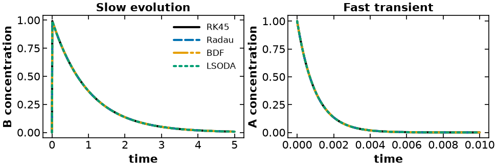

All four methods agree on the concentrations to better than 10^-7, but they do not need comparable work. In the tested course environment (scipy 1.18, and identical on 1.7):

method	kind	right-hand-side evaluations	accepted steps	LU factorizations	typical step after the transient
`RK45`	explicit	11,012	1,582	0	$3.3 \times 10^{-3}$
`Radau`	implicit	1,926	274	66	$5.6 \times 10^{-2}$
`BDF`	implicit	556	277	52	$7.9 \times 10^{-2}$
`LSODA`	switching	484	236	9	$7.3 \times 10^{-2}$

The mechanism is in the left panel of the figure: once the fast transient is over, the solution is a smooth exponential decay and accuracy alone would permit a large step. Radau, BDF and LSODA take one. RK45 cannot, because its step is capped by the fast eigenvalue $-k_1$ — still -1000 long after the mode it belongs to has died — at the Dormand--Prince stability limit $h \approx 3.3/k_1$ . The step it actually takes, $3.25 \times 10^{-3}$ , is that ceiling, not an accuracy requirement.

Exact counts depend on software version and tolerances; the qualitative gap — roughly twenty times the work for the same answer — is the lesson.

Discussion: Which method would you try first if this integration were repeated inside an optimization algorithm? What additional information would you check before deciding?

References¶

Biegler, L. T. (2010). Nonlinear Programming: Concepts, Algorithms, and Applications to Chemical Processes. Society for Industrial. 10.1137/1.9780898719383