Differential Algebraic Equations (DAEs) - Optimization for Decision Science

Prepared by: Prof. Alexander Dowling, Myia Dickens (mdicken2@nd.edu, 2023), Molly Dougher (mdoughe6@nd.edu, 2023)

This notebook follows one pendulum narrative: identify the DAE, expose its hidden constraints, observe why an index-3 formulation defeats a standard DAE integrator, and compare index-reduced alternatives. The goal is to prepare an integration-ready model for numerical integration and direct collocation.

import sys

if "google.colab" in sys.modules:
    !wget "https://raw.githubusercontent.com/ndcbe/optimization/main/notebooks/helper.py"
    !pip install casadi
    import helper

    helper.easy_install()
else:
    sys.path.insert(0, "../")
    import helper
helper.set_plotting_style()

Software used¶

Pyomo.DAE expresses differential and algebraic equations and can discretize them for optimization.
CasADi provides the interface used by Pyomo.DAE.Simulator; its idas plugin calls the SUNDIALS IDA integrator.

The notebook intentionally preserves one expected solver failure. A caught IDA_CONV_FAIL is evidence about the high-index formulation, not a notebook error.

DAE index and index reduction¶

Definition 8.6: Consider the DAE systems of the form:
$\begin{align} F\left(x, \frac{d x}{d t}, u(t), p, t\right)=0, \quad h(x(0))=0 \end{align}$
(1)
OR
$\frac{d z}{d t}= f(z(t), y(t), u(t), p), \quad z(0)=z_0, \quad g(z(t), y(t), u(t), p)=0$
(2)
with decisions $u(t)$ and $p$ fixed. The index is the integer $s$ that represents the minimum number of differentiations of the DAE system (with respect to time) required to determine an ODE for the variables $z(t)$ and $y(t)$ .

Generally, for semiexplicit systems, the index of a DAE system can be determined by first differentiating the algebraic equations and then substituting resulting differential terms into the respective differential equation. Recall the number of differentiations required to isolate an ODE system corresponds to the index.

As the goal is usually to isolate a DAE of index 1, the following algorithm describes the typical procedure to reduce the index of a DAE system.

Algorithm 8.1: (Reduction of High Index DAEs) Start with a DAE of the form:
$\frac{d z}{d t}= f(z(t), y(t), u(t), p), \quad z(0)=z_0, \quad g(z(t), y(t), u(t), p)=0.$
(3)
Check if the DAE system is index 1. If yes, stop.
Identify a subset of algebraic equations that can be solved for a subset of algebraic variables.
Consider the remaining algebraic equations that contain differential variables $z_j$ . Differentiating these remaining algebraic equations with respect to time leads to terms $\frac{dz_j}{dt}$ in the differentiated equations.
For the differential terms $\frac{dz_j}{dt}$ , substitute the right-hand sides of the corresponding differential equations $f_j(z,y,u,p)$ into the differentiated algebraic equations, and eliminate (some of) these differential equations. This leads to new algebraic equations that replace the same number of existing differential equations.
With this new DAE system, go to step 1.

An example of this algorithm in use can be found within the following pendulum example.

Pendulum model and index reduction¶

The pendulum follows Ascher and Petzold, Sections 1.3 and 9.1--9.2. We will use it to compare the original index-3 model with pure-ODE and index-1 reformulations.

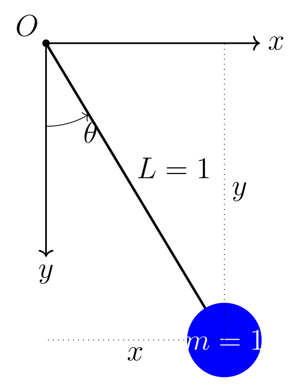
$Simple pendulum: mass m=1 on a rigid link of length L=1, with angle \theta from vertical.$

The following DAE system describes the pendulum system:

\begin{align} & x' = u \\ & y' = v \\ & u' = -Tx \\ & v' = g - Ty \\ & x^2 + y^2 = 1 \\ \end{align}

(4)

To find the index of the DAE system, first take the derivative of the algebraic equation and substitute in for the differential variables:

\begin{align} & x^2 + y^2 = 1 \\ & 2xx' + 2yy' = 0 \\ & 2xu + 2yv = 0 \end{align}

(5)

Next, differentiate the obtained equation using the product rule, make similar substitutions, and rearrange:

\begin{align} & 2xu + 2yv = 0 \\ & 2(xu'+ x'u) + 2(yv' + vy') = 0 \\ & 2(-Tx^2 + u^2) + 2(y(g-Ty) + v^2) = 0 \\ & 2(u^2 + v^2) + 2(-Tx^2 + gy - Ty^2) = 0 \\ & 2(u^2 + v^2) - 2T(x^2 + y^2) + 2gy = 0 \end{align}

(6)

Finally, implicitly differentiate the obtained equation, make similar substitutions, and rearrange to isolate the $T'$ term:

\begin{align} & 2(u^2 + v^2) - 2T(x^2 + y^2) + 2gy = 0 \\ & 4(uu' + vv') - 4T(xx' + yy') - 2T'(x^2 + y^2) + 2gy' = 0 \\ & 4(uu' + vv') - 4T(xx' + yy') + 2gy' = 2T'(x^2 + y^2) \\ & 4(-Tux + v(g-Ty)) - 4T(xu + yv) + 2gv = 2T' \\ & 4(-Tux -Tyv + gv) - 4T(xu + yv) + 2gv = 2T' \end{align}

(7)

Now the equations are a system of ODEs. Three differentiations were completed, indicating that this is an Index 3 DAE.

To reduce this DAE to index 1, follow Algorithm 8.1. The above analysis shows that this is not an index 1 DAE system. Therefore, the following algebraic equation is identified: $x^2 + y^2 = 1$ . Differentiate the algebraic equation to yield:

\begin{align} & 2xx' + 2yy' = 0\\ \end{align}

(8)

which can be solved for $x'$ . Substitute for $x'$ and $y'$ to yield:

\begin{align} & 2xu + 2yv = 0\\ \end{align}

(9)

The new DAE system is now:

\begin{align} & y' = v \\ & u' = -Tx \\ & v' = g - Ty \\ & x^2 + y^2 = 1 \\ & 2xu + 2yv = 0 \\ \end{align}

(10)

where $x$ is now an algebraic variable and the final equation must be solved for $T$ . Differentiating the algebraic (last) equation leads to:

\begin{align} & 2(xu'+ x'u) + 2(yv' + vy') = 0 \\ & 2(xu' + u^2) + 2(yv' + v^2) = 0 \\ & 2(u^2 - Tx^2) + 2(v^2 + gy - Ty^2) = 0 \\ \end{align}

(11)

The equations can replace $u' = -Tx$ , leading to the following DAE system:

\begin{align} & y' = v \\ & v' = g - Ty \\ & x^2 + y^2 = 1 \\ & 2xu + 2yv = 0 \\ & (u^2 + v^2) - T\underbrace{(x^2 + y^2)}_{1} + gy = 0 \\ \end{align}

(12)

which is an Index 1 DAE.

## Load libraries
import pyomo.environ as pyo
import pyomo.dae as dae
from pyomo.dae.simulator import Simulator
import matplotlib.pyplot as plt
import numpy as np


## Define function for plotting results
def plot_results(sim, tsim, profiles):
    """
    inputs:

    sim: pyomo.DAE simulator results from a simulation of ODE or DAE
    tsim: 1D array of time samples of the DAE/ODE simulatiion
    profiles: 2D array of simulated differential and algebraic equations

    outputs:

    Plot 1: A plot of the curated profiles
    Plot 2: A plot of the simulated results

    time = list(m.t)
    x = [value(m.x[t]) for t in m.t]
    y = [value(m.y[t]) for t in m.t]

    plt.plot(time, x, '-b', label='x')
    plt.plot(time, y, '-r', label='y')
    plt.xlabel('Time')
    plt.ylabel('Position')
    plt.legend(loc='best')
    plt.show()
    """

    plt.figure(1, figsize=(4, 4))

    # Every series also carries a linestyle, so the figure survives a
    # black-and-white printout (figures/README.md).
    linestyles = ["-", "--", "-.", ":", (0, (3, 1, 1, 1, 1, 1))]

    varorder = sim.get_variable_order()
    algorder = sim.get_variable_order(vartype="algebraic")

    # Create empty dictionary
    results = {}

    # Collect Different Profiles
    for idx1, v in enumerate(varorder):
        i = idx1
        v_ = str(v)
        results[v_] = profiles[:, i]
        plt.plot(tsim, results[v_], label=v, linestyle=linestyles[i % len(linestyles)])

    # Collect Algebraic Profiles
    for idx2, v in enumerate(algorder):
        i = len(varorder) + idx2
        v_ = str(v)
        results[v_] = profiles[:, i]
        plt.plot(tsim, results[v_], label=v, linestyle=linestyles[i % len(linestyles)])

    # Plot the simulated algebraic and differential profiles as they change in time
    plt.xlabel("t", fontsize=16, fontweight="bold")
    plt.tick_params(direction="in", labelsize=15)
    plt.legend(loc="best")

    plt.show()

    # Plot the results of the simulation
    plt.figure(2, figsize=(4, 4))
    x_ = results["x[{t}]"]
    y_ = results["y[{t}]"]
    plt.plot(tsim, np.sqrt(x_**2 + y_**2), "-b", label="length")
    plt.xlabel("t", fontsize=16, fontweight="bold")
    plt.tick_params(direction="in", labelsize=15)
    plt.ylabel(r"$\sqrt{x^2 + y^2}$")
    plt.show()

    # return results

Formulation 1: Index-3 DAE¶

Consider the following model:

\begin{align} \frac{d x}{dt} &= u \\ \frac{d y}{dt} &= v \\ \frac{d u}{dt} &= -T x \\ \frac{d v}{dt} &= g - Ty \\ & x^2 + y^2 = 1 \end{align}

(13)

This assumes mass and length of unity.

Why this notebook does not carry Pyomo units.

The other notebooks in this section declare units= on every Var and Param and check with assert_units_consistent -- see Units in Pyomo.dae Models. This one deliberately does not, and the reason is worth stating rather than hiding.

The pendulum here is normalized: mass and length are both set to unity, so the constraint is written $x^2 + y^2 = 1$ against a dimensionless literal, and the “tension” $T$ is not a force. Reading $\frac{du}{dt} = -Tx$ dimensionally forces

[T] = \frac{\mathrm{m}/\mathrm{s}^2}{\mathrm{m}} = \mathrm{s}^{-2},

(14)

i.e. $T$ is really a tension divided by $mL$ . Restoring dimensions would mean rewriting $x^2 + y^2 = 1$ as $x^2 + y^2 = L^2$ and carrying $mL$ through the index reduction -- changing the very equations whose algebraic structure is the lesson of this notebook.

So: no units here, on purpose. A forced, arbitrary set of units is worse than none, because it produces a check that looks meaningful and is not.

That said, dimensional analysis by hand still pays -- see the next section.

def create_model_index3():
    """
    Creates a model to define the Index 3 DAE system.

    Output: the model, m
    """

    m = pyo.ConcreteModel()

    # Declare time
    m.t = dae.ContinuousSet(bounds=(0.0, 1))

    # Declare parameter - acceleration due to gravity
    m.g = pyo.Param(initialize=9.81)  # [m/s^2]

    # Declare variables indexed over time
    m.x = pyo.Var(m.t)  # horizontal position
    m.y = pyo.Var(m.t)  # vertical position
    m.u = pyo.Var(m.t)  # horizontal velocity
    m.v = pyo.Var(m.t)  # vertical velocity
    m.T = pyo.Var(m.t)  # tension

    # Four DerivativeVars: x, y, u and v all get one. Compare the index-1
    # model, which declares only two. Nothing below records that this system is
    # index 3 -- Pyomo has no notion of index, so the failure arrives at RUN
    # time, not build time: IDAS is written for index 0 and 1 and returns
    # IDA_CONV_FAIL at t = 0.
    # Declare derivative variables
    m.dx = dae.DerivativeVar(m.x)  # with respect to t is implied
    m.dy = dae.DerivativeVar(m.y)
    m.du = dae.DerivativeVar(m.u)
    m.dv = dae.DerivativeVar(m.v)

    # Declare differential equations
    @m.Constraint(m.t)
    def dx_eqn(m, t):
        return m.dx[t] == m.u[t]

    @m.Constraint(m.t)
    def dy_eqn(m, t):
        return m.dy[t] == m.v[t]

    @m.Constraint(m.t)
    def du_eqn(m, t):
        return m.du[t] == -m.T[t] * m.x[t]

    @m.Constraint(m.t)
    def dv_eqn(m, t):
        return m.dv[t] == m.g - m.T[t] * m.y[t]

    # Declare algebraic equation
    @m.Constraint(m.t)
    def alg_eqn(m, t):
        return m.x[t] ** 2 + m.y[t] ** 2 == 1

    # Specify initial conditions
    m.x[0] = 0
    m.y[0] = 1
    m.u[0] = 1
    m.v[0] = 0
    m.T[0] = 1 + m.g

    return m

index3 = create_model_index3()

# Specify integrator options
int_ops = {"print_stats": True, "abstol": 1e-8, "reltol": 1e-6}

# Solve DAEs
sim = Simulator(index3, package="casadi")
try:
    tsim, profiles = sim.simulate(
        numpoints=100, integrator="idas", integrator_options=int_ops
    )
except RuntimeError:
    # Expected: IDAS supports index-0 and index-1 DAEs, not this index-3 model.
    print("Expected IDAS failure: IDA_CONV_FAIL for the unreduced index-3 pendulum.")
else:
    plot_results(sim, tsim, profiles)

Expected IDAS failure: IDA_CONV_FAIL for the unreduced index-3 pendulum.

CasADi - 2026-09-07 10:56:45 WARNING("The options 't0', 'tf', 'grid' and 'output_t0' have been deprecated.
The same functionality is provided by providing additional input arguments to the 'integrator' function, in particular:
 * Call integrator(..., t0, tf, options) for a single output time, or
 * Call integrator(..., t0, grid, options) for multiple grid points.
The legacy 'output_t0' option can be emulated by including or excluding 't0' in 'grid'.
Backwards compatibility is provided in this release only.") [.../casadi/core/integrator.cpp:698]
At t = 0 and h = 1.06624e-14, the corrector convergence failed repeatedly or with |h| = hmin.

IDA solves implicit DAEs in residual form and is intended for index-1 systems. Here it repeatedly fails the corrector at $t=0$ and returns IDA_CONV_FAIL; reducing the model to index 0 or 1 is part of the modeling workflow, not a change of tolerances. See the SUNDIALS IDA documentation.

Formulation 2: Pure ODE Model/ Index-0 Example¶

\begin{align} \frac{d x}{dt} &= u \\ \frac{d y}{dt} &= v \\ \frac{d u}{dt} &= -T x \\ \frac{d v}{dt} &= g - Ty \\ \frac{d T}{dt} &= \frac{-4T(xu+yv)+3gv}{x^2+y^2} \end{align}

(15)

def create_model_ode():
    """
    Creates a model to define the Index 0 DAE system.

    Output: the model, m
    """

    m = pyo.ConcreteModel()

    # Declare time
    m.t = dae.ContinuousSet(bounds=(0.0, 5.0))

    # Declare parameter - acceleration due to gravit
    m.g = pyo.Param(initialize=9.81)  # [m/s^2]

    # Declare variables indexed over time
    m.x = pyo.Var(m.t)  # horizontal position
    m.y = pyo.Var(m.t)  # vertical position
    m.u = pyo.Var(m.t)  # horizontal velocity
    m.v = pyo.Var(m.t)  # vertical velocity
    m.T = pyo.Var(m.t)  # tension

    # Declare derivative variables
    m.dx = dae.DerivativeVar(m.x)  # with respect to t is implied
    m.dy = dae.DerivativeVar(m.y)
    m.du = dae.DerivativeVar(m.u)
    m.dv = dae.DerivativeVar(m.v)
    m.dT = dae.DerivativeVar(m.T)

    # Declare differential equations
    @m.Constraint(m.t)
    def dx_eqn(m, t):
        return m.dx[t] == m.u[t]

    @m.Constraint(m.t)
    def dy_eqn(m, t):
        return m.dy[t] == m.v[t]

    @m.Constraint(m.t)
    def du_eqn(m, t):
        return m.du[t] == -m.T[t] * m.x[t]

    @m.Constraint(m.t)
    def dv_eqn(m, t):
        return m.dv[t] == m.g - m.T[t] * m.y[t]

    @m.Constraint(m.t)
    def dT_eqn(m, t):
        return (
            m.dT[t]
            == (
                -4 * m.T[t] * (m.x[t] * m.u[t] + m.y[t] * m.v[t])
                + 3 * m.g * m.v[t]
            ) / (m.x[t] ** 2 + m.y[t] ** 2)
        )

    # Specify initial conditions
    m.x[0] = 0
    m.y[0] = 1
    m.u[0] = 1
    m.v[0] = 0
    m.T[0] = 1 + m.g

    return m


ode = create_model_ode()

# Specify integrator options
int_ops = {"print_stats": True, "abstol": 1e-6, "reltol": 1e-4}

# Solve DAEs
sim = Simulator(ode, package="casadi")
tsim, profiles = sim.simulate(
    numpoints=100, integrator="idas", integrator_options=int_ops
)

# Plot solution
results = plot_results(sim, tsim, profiles)

FORWARD INTEGRATION:
Number of steps taken by SUNDIALS: 172
Number of calls to the user's f function: 236
Number of calls made to the linear solver setup function: 25
Number of error test failures: 6
Method order used on the last internal step: 5
Method order to be used on the next internal step: 5
Actual value of initial step size: 7.90569e-07
Step size taken on the last internal step: 0.0158106
Step size to be attempted on the next internal step: 0.0316212
Current internal time reached: 5
Number of nonlinear iterations performed: 234
Number of nonlinear convergence failures: 0

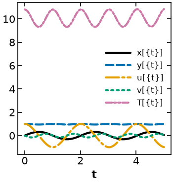
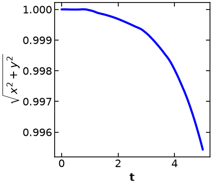
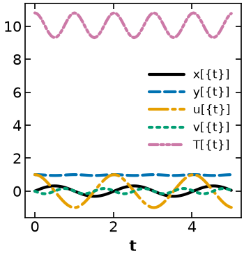
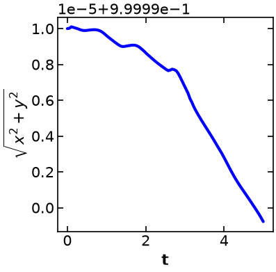
The drift, over a longer horizon¶

The plot above is the same quantity as the figure below, run for $t \in [0, 5]$ with IDAS. The figure below is the canonical version used in the lecture handout: the same index-reduced ODE, integrated with scipy.integrate.solve_ivp (RK45) out to $t = 50$ , at two tolerances, and with a third curve that adds the stabilization term $-\gamma F(x) h(x)$ of Ascher & Petzold (1998), eq. (9.40), p. 251.

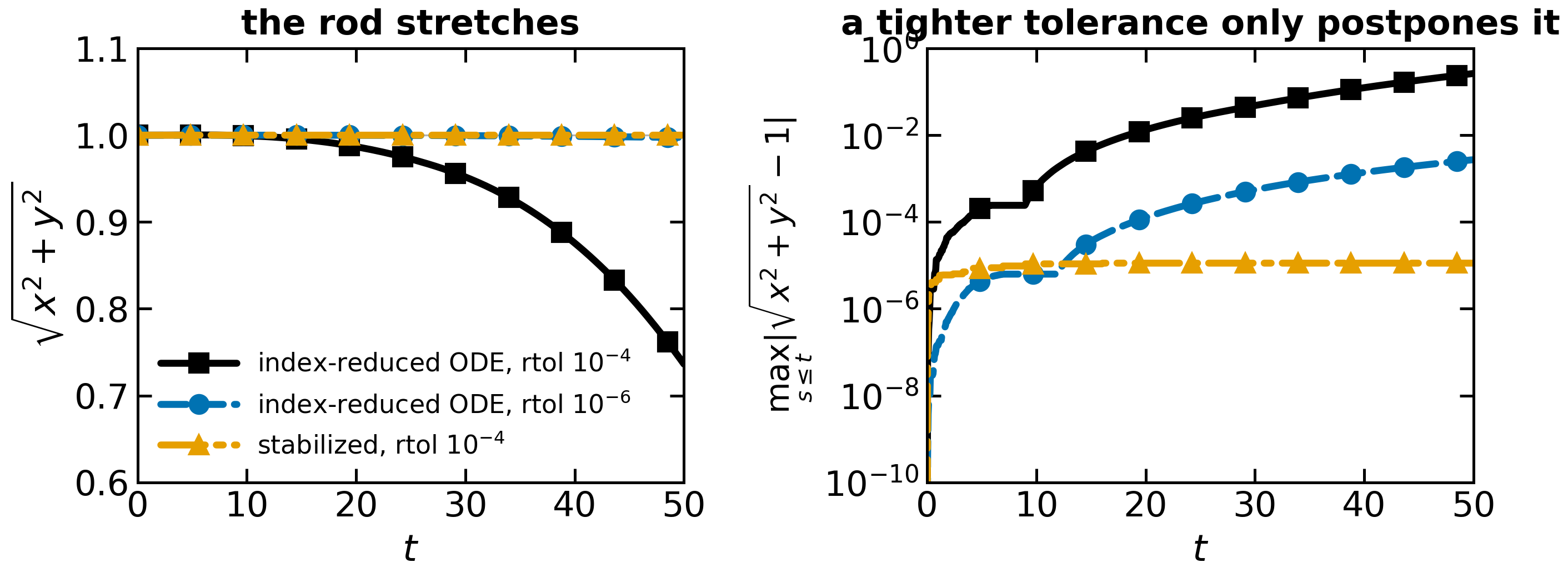
Drift off the constraint manifold for the index-reduced pendulum

The takeaway: drift is not a tolerance bug. Tightening rtol buys decades, not a fix, because nothing in the reduced ODE refers to $x^2 + y^2 = 1$ — only to its derivatives.

Source: figures/plots/pendulum-drift.py. The figure and Pyomo model both use $\dot T = [-4T(xu+yv) + 3gv]/(x^2+y^2)$ , obtained by differentiating the acceleration constraint.

Dimensional check¶

Restore units: $x,y$ in m; $u,v$ in m/s; and $T$ in $\mathrm{s}^{-2}$ .

Term	Units
$-4T(xu+yv)+3gv$	$\mathrm{m}^2\,\mathrm{s}^{-3}$
$x^2+y^2$	$\mathrm{m}^2$
quotient, $\dot T$	$\mathrm{s}^{-3}$

The denominator is required dimensionally. Normalizing the rod length to one can hide this factor algebraically, but not physically.

Discussion

Are all of the algebraic constraints in the original formulation satisfied?

Formulation 3: Index-1 DAE Model¶

\begin{align} \frac{d y}{dt} &= v \\ \frac{d v}{dt} &= g - Ty \\ & x^2 + y^2 = 1 \\ & 2 x u + 2 y v = 0 \\ & (u^2 + v^2) - T \underbrace{(x^2 + y^2)}_{1} + g y = 0 \end{align}

(16)

(This reformulation is NOT unique... could have written $\frac{dx}{dt}$ and $\frac{du}{dt}$ instead.)

Consistent initial conditions:

Specify $y(0)$ and $v(0)$ .
Solve for $x(0)$ , $u(0)$ , and $T(0)$

def create_model_index1():
    """
    Creates a model to define the Index 1 DAE system.

    Output: the model, m
    """

    m = pyo.ConcreteModel()

    # Declare time
    m.t = dae.ContinuousSet(bounds=(0, 5))

    # Declare parameter - acceleration due to gravity
    m.g = pyo.Param(initialize=9.81)  # [m/s^2]

    # Declare variables indexed over time
    m.x = pyo.Var(m.t)  # horizontal position
    m.y = pyo.Var(m.t)  # vertical position
    m.u = pyo.Var(m.t)  # horizontal velocity
    m.v = pyo.Var(m.t)  # vertical velocity
    m.T = pyo.Var(m.t)  # tension

    # THIS is what makes the formulation index 1, and it is the only thing
    # that does: two DerivativeVars where the index-3 model had four. The
    # algebraic and differential equations are all pyo.Constraint over m.t --
    # the modeling language does not distinguish them. Which variables get a
    # derivative is the modeling choice.
    m.dy = dae.DerivativeVar(m.y)
    m.dv = dae.DerivativeVar(m.v)

    # Declare differential equations
    @m.Constraint(m.t)
    def dy_eqn(m, t):
        return m.dy[t] == m.v[t]

    @m.Constraint(m.t)
    def dv_eqn(m, t):
        return m.dv[t] == m.g - m.T[t] * m.y[t]

    # Declare algebraic equations
    @m.Constraint(m.t)
    def alg_eqn1(m, t):
        return m.x[t] ** 2 + m.y[t] ** 2 == 1

    @m.Constraint(m.t)
    def alg_eqn2(m, t):
        return m.x[t] * m.u[t] + m.y[t] * m.v[t] == 0

    @m.Constraint(m.t)
    def alg_eqn3(m, t):
        return (
            m.u[t] ** 2
            + m.v[t] ** 2
            - m.T[t] * (m.x[t] ** 2 + m.y[t] ** 2)
            + m.g * m.y[t]
            == 0
        )

    # Specify initial conditions
    m.x[0] = 0
    m.y[0] = 1
    m.u[0] = 1
    m.v[0] = 0
    m.T[0] = 1 + m.g

    return m

def index1_check_constraints(m):
    """Check if the three constraints are feasible."""

    print("Constraint 1:")
    r1 = m.x[0]() ** 2 + m.y[0]() ** 2 - 1
    print(r1)

    print("\nConstraint 2:")
    r2 = m.x[0]() * m.u[0]() + m.y[0]() * m.v[0]()
    print(r2)

    print("\nConstraint 3:")
    r3 = m.u[0]() ** 2 + m.v[0]() ** 2 - m.T[0]() + m.g * m.y[0]()
    print(r3)


index1 = create_model_index1()

# Check initial condition
index1_check_constraints(index1)

# Specify integrator options
int_ops = {"print_stats": True, "abstol": 1e-6, "reltol": 1e-4}

# Solve DAEs
sim = Simulator(index1, package="casadi")
try:
    tsim, profiles = sim.simulate(
        numpoints=100, integrator="idas", integrator_options=int_ops
    )
except RuntimeError as err:
    # Expected here: the reformulation is singular at x = 0.
    print(f"Expected point-singularity failure: {err}")
# tsim, profiles = sim.simulate(numpoints=100, integrator='collocation')

Constraint 1:
0

Constraint 2:
0

Constraint 3:
0.0
Expected point-singularity failure: Error in Function::call for 'F' [IdasInterface] at .../casadi/core/function.cpp:1466:
Error in Function::call for 'F' [IdasInterface] at .../casadi/core/function.cpp:362:
.../casadi/interfaces/sundials/idas_interface.cpp:599: IDACalcIC returned "IDA_NO_RECOVERY". Consult IDAS documentation.

The residual routine or the linear setup or solve routine had a recoverable error, but IDACalcIC was unable to recover.

What happened? The chosen algebraic equation--variable pairing is singular at $x=0$ .

Let’s try $x=0.1$ as the initial point.

index1_again = create_model_index1()

# Specify alternative initial conditions
small_number = 0.1

index1_again.x[0] = small_number
index1_again.y[0] = 1
index1_again.u[0] = 1
index1_again.v[0] = 0
index1_again.T[0] = 1 + index1_again.g

# Check initial condition
index1_check_constraints(index1_again)

# Solve DAEs
sim = Simulator(index1_again, package="casadi")

# Simulator
try:
    tsim, profiles = sim.simulate(
        numpoints=100, integrator="idas", integrator_options=int_ops
    )
except RuntimeError as err:
    # Expected here: these trial initial values violate the invariants.
    print(f"Expected inconsistent-initialization failure: {err}")

Constraint 1:
0.010000000000000009

Constraint 2:
0.1

Constraint 3:
0.0
Expected inconsistent-initialization failure: Error in Function::call for 'F' [IdasInterface] at .../casadi/core/function.cpp:1466:
Error in Function::call for 'F' [IdasInterface] at .../casadi/core/function.cpp:362:
.../casadi/interfaces/sundials/idas_interface.cpp:599: IDACalcIC returned "IDA_NO_RECOVERY". Consult IDAS documentation.

The residual routine or the linear setup or solve routine had a recoverable error, but IDACalcIC was unable to recover.

Our initial point does not satisfy the algebraic constraints! We need a consistent initial point.

Given $x = \epsilon$ , solve $x^2 + y^2 = 1$ for $y$ :

y = \sqrt{1^2 - \epsilon^2}

(17)

Then, assume $u = 1$ and solve $2 x u + 2 y v = 0$ for $v$ :

v = \frac{-x u}{y}

(18)

Finally, we can solve $(u^2 + v^2) - T (x^2 + y^2) + g y = 0$ for $T$ :

T = \frac{(u^2 + v^2) + gy}{x^2 + y^2} = \frac{(u^2 + v^2) + gy}{1}

(19)

index1_take_two = create_model_index1()

# Specify alternative initial conditions
small_number = 0.1

index1_take_two.x[0] = small_number
index1_take_two.y[0] = np.sqrt(1 - small_number**2)
index1_take_two.u[0] = 1
index1_take_two.v[0] = (
    -index1_take_two.x[0]() * index1_take_two.u[0]() / index1_take_two.y[0]()
)
index1_take_two.T[0] = (
    index1_take_two.u[0]() ** 2
    + index1_take_two.v[0]() ** 2
    + index1_take_two.g * index1_take_two.y[0]()
)

# Check initial condition
index1_check_constraints(index1_take_two)

# Solve DAEs
sim = Simulator(index1_take_two, package="casadi")

# Specify integrator options
int_ops2 = {
    "print_stats": True,
    "abstol": 1e-6,
    "reltol": 1e-4,
    "verbose": False,
    "calc_ic": True,
}

# Simulator
try:
    tsim, profiles = sim.simulate(
        numpoints=20, integrator="idas", integrator_options=int_ops2
    )
except RuntimeError as err:
    # This documented failure motivates discretizing the model next.
    print(f"Expected formulation failure: {err}")

Constraint 1:
0.0

Constraint 2:
0.0

Constraint 3:
0.0
Expected formulation failure: Error in Function::call for 'F' [IdasInterface] at .../casadi/core/function.cpp:1466:
Error in Function::call for 'F' [IdasInterface] at .../casadi/core/function.cpp:362:
.../casadi/interfaces/sundials/idas_interface.cpp:599: IDACalcIC returned "IDA_NO_RECOVERY". Consult IDAS documentation.

The residual routine or the linear setup or solve routine had a recoverable error, but IDACalcIC was unable to recover.

The trajectory is still not reliable: this formulation has a point singularity.

Let’s try solving the model with Ipopt after discretizing with collocation.

# discretize the model
index1_take_two.Obj = pyo.Objective(expr=1)  # Add a dummy objective
discretizer = pyo.TransformationFactory("dae.collocation")
discretizer.apply_to(index1_take_two, nfe=15, scheme="LAGRANGE-RADAU", ncp=3)

# initialize
for t in index1_take_two.t:
    index1_take_two.x[t] = small_number
    index1_take_two.y[t] = np.sqrt(1 - small_number**2)
    index1_take_two.u[t] = 1
    index1_take_two.v[t] = (
        -index1_take_two.x[t]() * index1_take_two.u[t]() / index1_take_two.y[t]()
    )
    index1_take_two.T[t] = (
        index1_take_two.u[t]() ** 2
        + index1_take_two.v[t]() ** 2
        + index1_take_two.g * index1_take_two.y[t]()
    )

# solve the discretized model
solver = pyo.SolverFactory("ipopt")
solver.options["max_iter"] = 300
results = solver.solve(index1_take_two, tee=True)
assert pyo.check_optimal_termination(results), (
    f"Solve failed: status={results.solver.status}, "
    f"termination={results.solver.termination_condition}"
)

Ipopt 3.14.19: max_iter=300


******************************************************************************
This program contains Ipopt, a library for large-scale nonlinear optimization.
 Ipopt is released as open source code under the Eclipse Public License (EPL).
         For more information visit https://github.com/coin-or/Ipopt
******************************************************************************

This is Ipopt version 3.14.19, running with linear solver MUMPS 5.8.2.

Number of nonzeros in equality constraint Jacobian...:     1186
Number of nonzeros in inequality constraint Jacobian.:        0
Number of nonzeros in Lagrangian Hessian.............:      368

Total number of variables............................:      322
                     variables with only lower bounds:        0
                variables with lower and upper bounds:        0
                     variables with only upper bounds:        0
Total number of equality constraints.................:      320
Total number of inequality constraints...............:        0
        inequality constraints with only lower bounds:        0
   inequality constraints with lower and upper bounds:        0
        inequality constraints with only upper bounds:        0

iter    objective    inf_pr   inf_du lg(mu)  ||d||  lg(rg) alpha_du alpha_pr  ls
   0  1.0000000e+00 9.07e-01 0.00e+00  -1.0 0.00e+00    -  0.00e+00 0.00e+00   0

   1  1.0000000e+00 2.58e+00 1.51e-21  -1.7 4.10e+00    -  1.00e+00 1.00e+00h  1

   2  1.0000000e+00 3.54e+00 9.17e-03  -1.7 2.11e+00  -4.0 1.00e+00 1.00e+00h  1

   3  1.0000000e+00 3.17e+00 2.87e-01  -1.7 1.78e+00  -3.6 1.00e+00 1.00e+00h  1
   4  1.0000000e+00 6.54e-01 7.16e-02  -1.7 2.49e+00    -  1.00e+00 1.00e+00h  1
   5  1.0000000e+00 1.56e-01 1.79e-02  -1.7 3.95e-01  -3.1 1.00e+00 1.00e+00h  1

   6  1.0000000e+00 3.66e-02 4.48e-03  -2.5 1.92e-01  -2.7 1.00e+00 1.00e+00h  1

   7  1.0000000e+00 1.87e-02 5.74e-02  -2.5 2.25e-01  -2.3 1.00e+00 5.00e-01h  2

   8  1.0000000e+00 1.84e-02 1.44e-02  -2.5 1.39e-01    -  1.00e+00 1.00e+00h  1
   9  1.0000000e+00 5.18e-03 3.59e-03  -3.8 7.39e-02    -  1.00e+00 1.00e+00h  1
iter    objective    inf_pr   inf_du lg(mu)  ||d||  lg(rg) alpha_du alpha_pr  ls
  10  1.0000000e+00 1.30e-03 8.97e-04  -3.8 3.69e-02    -  1.00e+00 1.00e+00h  1

  11  1.0000000e+00 3.24e-04 2.24e-04  -5.7 1.85e-02    -  1.00e+00 1.00e+00h  1
  12  1.0000000e+00 8.10e-05 5.61e-05  -5.7 9.23e-03    -  1.00e+00 1.00e+00h  1
  13  1.0000000e+00 2.02e-05 1.40e-05  -5.7 4.62e-03    -  1.00e+00 1.00e+00h  1
  14  1.0000000e+00 5.06e-06 3.50e-06  -5.7 2.31e-03    -  1.00e+00 1.00e+00h  1

  15  1.0000000e+00 1.26e-06 8.76e-07  -8.6 1.15e-03    -  1.00e+00 1.00e+00h  1
  16  1.0000000e+00 3.16e-07 2.19e-07  -8.6 5.77e-04    -  1.00e+00 1.00e+00h  1
  17  1.0000000e+00 7.91e-08 5.48e-08  -8.6 2.88e-04    -  1.00e+00 1.00e+00h  1

  18  1.0000000e+00 1.98e-08 1.37e-08  -8.6 1.44e-04    -  1.00e+00 1.00e+00h  1
  19  1.0000000e+00 4.94e-09 3.42e-09  -9.0 7.21e-05    -  1.00e+00 1.00e+00h  1

Number of Iterations....: 19

                                   (scaled)                 (unscaled)
Objective...............:   1.0000000000000000e+00    1.0000000000000000e+00
Dual infeasibility......:   3.4227968138033751e-09    3.4227968138033751e-09
Constraint violation....:   4.9411463920456812e-09    4.9411463920456812e-09
Variable bound violation:   0.0000000000000000e+00    0.0000000000000000e+00
Complementarity.........:   0.0000000000000000e+00    0.0000000000000000e+00
Overall NLP error.......:   4.9411463920456812e-09    4.9411463920456812e-09


Number of objective function evaluations             = 22
Number of objective gradient evaluations             = 20
Number of equality constraint evaluations            = 22
Number of inequality constraint evaluations          = 0
Number of equality constraint Jacobian evaluations   = 20
Number of inequality constraint Jacobian evaluations = 0
Number of Lagrangian Hessian evaluations             = 19
Total seconds in IPOPT                               = 0.515

EXIT: Optimal Solution Found.

Takeaway: Formulation 3 has a point singularity that defeats this integration attempt. Direct collocation can still solve the discretized model, but reformulation quality remains important.

Formulation 4: Index-1 DAE Model¶

\begin{align} \frac{d x}{dt} &= u \\ \frac{d y}{dt} &= v \\ \frac{d u}{dt} &= -T x \\ \frac{d v}{dt} &= g - Ty \\ 0 &= (u^2 + v^2) - T (x^2 + y^2) + g y \end{align}

(20)

Consistent initial conditions:

Specify $x(0)$ , $u(0)$ , $y(0)$ , and $v(0)$ .
Solve for $T(0)$

def create_model_index1_b():
    """
    Creates a model to define the Index 1 DAE system.

    Output: the model, m
    """

    m = pyo.ConcreteModel()

    # Declare time
    m.t = dae.ContinuousSet(bounds=(0.0, 5))

    # Declare parameter - acceleration due to gravity
    m.g = pyo.Param(initialize=9.81)  # [m/s^2]

    # Declare variables indexed over time
    m.x = pyo.Var(m.t)  # horizontal position
    m.y = pyo.Var(m.t)  # vertical position
    m.u = pyo.Var(m.t)  # horizontal velocity
    m.v = pyo.Var(m.t)  # vertical velocity
    m.T = pyo.Var(m.t)  # tension

    # Declare derivative variables
    m.dx = dae.DerivativeVar(m.x)  # with respect to t is implied
    m.dy = dae.DerivativeVar(m.y)
    m.du = dae.DerivativeVar(m.u)
    m.dv = dae.DerivativeVar(m.v)

    # Declare differential equations
    @m.Constraint(m.t)
    def dx_eqn(m, t):
        return m.dx[t] == m.u[t]

    @m.Constraint(m.t)
    def dy_eqn(m, t):
        return m.dy[t] == m.v[t]

    @m.Constraint(m.t)
    def du_eqn(m, t):
        return m.du[t] == -m.T[t] * m.x[t]

    @m.Constraint(m.t)
    def dv_eqn(m, t):
        return m.dv[t] == m.g - m.T[t] * m.y[t]

    @m.Constraint(m.t)
    def alg_eqn3(m, t):
        return (
            m.u[t] ** 2
            + m.v[t] ** 2
            - m.T[t] * (m.x[t] ** 2 + m.y[t] ** 2)
            + m.g * m.y[t]
            == 0
        )

    # Specify initial conditions
    m.x[0] = 0
    m.y[0] = 1
    m.u[0] = 1
    m.v[0] = 0
    m.T[0] = 1 + m.g

    return m

index1_b = create_model_index1_b()

# Specify integrator options
int_ops = {"print_stats": True, "abstol": 1e-8, "reltol": 1e-6}

# Solve DAEs
sim = Simulator(index1_b, package="casadi")
tsim, profiles = sim.simulate(
    numpoints=100, integrator="idas", integrator_options=int_ops
)

# Plot solution
plot_results(sim, tsim, profiles)

FORWARD INTEGRATION:
Number of steps taken by SUNDIALS: 379
Number of calls to the user's f function: 485
Number of calls made to the linear solver setup function: 31
Number of error test failures: 3
Method order used on the last internal step: 5
Method order to be used on the next internal step: 5
Actual value of initial step size: 7.90569e-09
Step size taken on the last internal step: 0.0120796
Step size to be attempted on the next internal step: 0.0120796
Current internal time reached: 5
Number of nonlinear iterations performed: 483
Number of nonlinear convergence failures: 0

Does the reformulation actually hold the constraint?¶

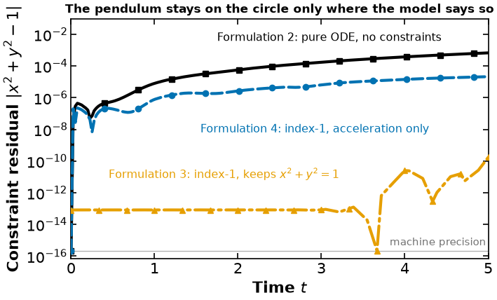
Formulation 2 integrates, but nothing in it refers to $x^2 + y^2 = 1$ — only to derivatives of it — so the bob slowly leaves the circle. The figure below is the numerical answer to the discussion question above, measured as the constraint residual

r(t) = \left| x(t)^2 + y(t)^2 - 1 \right|,

(21)

which is zero exactly when the rod has its original length. Three formulations are compared over the same horizon $t \in [0, 5]$ :

Series	What the model contains	How it is solved
Formulation 2, index-reduced ODE	no algebraic equations at all	`IDAS`, `abstol` 10^-8 / `reltol` 10^-6
Formulation 4, index-1 DAE	the acceleration-level constraint only	`IDAS`, same tolerances
Formulation 3, index-1 DAE	$x^2 + y^2 = 1$ itself, plus its first two derivatives	direct collocation + Ipopt (the solve above)

⚠ Read the middle series carefully: reaching index 1 is not by itself the fix. Formulation 4 is index 1 and still drifts, because the constraint it kept is not the one being measured. Only Formulation 3, which carries $x^2 + y^2 = 1$ as an equation of the model, holds it — there to solver tolerance, and flat in time rather than growing.

# ---------- SOLVE + EXTRACT ------------------------------------------------
# Everything below this cell reads `results` and nothing else. The archive
# figures/results/pendulum-index1-residual.json stores the DATA -- three time
# series of the constraint residual -- so the figure can be restyled later
# without CasADi, IDAS or Ipopt. See figures/README.md and
# figures/render_from_notebook.py for the cell contract.
#
# `source_tag` points at `handout:pendulum-index1` (Formulation 3, the model
# that keeps x^2 + y^2 = 1), so scripts/check_results_fresh.py reports it when
# that model changes and these numbers do not.
#
# ⚠ BOTH INTEGRATIONS USE THE TIGHTER TOLERANCE PAIR (1e-8 / 1e-6), not the
# 1e-6 / 1e-4 used earlier in the notebook for Formulation 2. That is
# deliberate: the point of the figure is that drift is a property of the
# formulation, so the loose tolerance must not be available as an explanation.


def residual_from_simulation(m, int_ops, numpoints=200):
    """|x^2 + y^2 - 1| along an IDAS simulation of `m`. Returns (t, residual)."""
    sim = Simulator(m, package="casadi")
    tsim, profiles = sim.simulate(
        numpoints=numpoints, integrator="idas", integrator_options=int_ops
    )
    # Column order is whatever the Simulator reports, not the order the model
    # declares -- ask it rather than assuming.
    order = [str(v) for v in sim.get_variable_order()]
    order += [str(v) for v in sim.get_variable_order(vartype="algebraic")]
    col = {name: k for k, name in enumerate(order)}
    x = profiles[:, col["x[{t}]"]]
    y = profiles[:, col["y[{t}]"]]
    return (
        [float(t) for t in tsim],
        [float(abs(xi**2 + yi**2 - 1.0)) for xi, yi in zip(x, y)],
    )


def residual_from_discretized(m):
    """|x^2 + y^2 - 1| at every collocation point of a solved model."""
    ts = sorted(m.t)
    return (
        [float(t) for t in ts],
        [float(abs(m.x[t]() ** 2 + m.y[t]() ** 2 - 1.0)) for t in ts],
    )


tight = {"abstol": 1e-8, "reltol": 1e-6}

t_ode, r_ode = residual_from_simulation(create_model_ode(), tight)
t_i1b, r_i1b = residual_from_simulation(create_model_index1_b(), tight)
# Formulation 3, already discretized and solved with Ipopt above.
t_col, r_col = residual_from_discretized(index1_take_two)

results = {
    # The residual floor. A residual is exactly 0.0 at t = 0 for every series
    # (the initial conditions are consistent), and 0 has no place on a log
    # axis. The floor is machine epsilon, which is also the smallest residual
    # that means anything here; the plotting cell clips to it and the axis
    # label says so.
    "floor": 2.220446049250313e-16,
    "series": [
        {
            "key": "ode",
            "label": "Formulation 2: pure ODE, no constraints",
            "note": "no algebraic equations; IDAS",
            "t": t_ode,
            "residual": r_ode,
        },
        {
            "key": "index1_accel",
            "label": "Formulation 4: index-1, acceleration only",
            "note": "keeps only $u^2+v^2-T(x^2+y^2)+gy=0$; IDAS",
            "t": t_i1b,
            "residual": r_i1b,
        },
        {
            "key": "index1_position",
            "label": "Formulation 3: index-1, keeps $x^2+y^2=1$",
            "note": "direct collocation, %d finite elements; Ipopt" % 15,
            "t": t_col,
            "residual": r_col,
        },
    ],
}

for s in results["series"]:
    print(f"{s['key']:>16s}: max residual = {max(s['residual']):.2e}")

helper.save_results(
    "pendulum-index1-residual",
    results,
    notebook="notebooks/3-dev/DAE_background.ipynb",
    source_tag="handout:pendulum-index1",
    description=(
        "Constraint residual |x^2 + y^2 - 1| for the pendulum over t in [0, 5], "
        "for the index-reduced pure ODE (Formulation 2), the index-1 DAE that "
        "keeps only the acceleration constraint (Formulation 4), and the index-1 "
        "DAE that keeps x^2 + y^2 = 1 itself (Formulation 3, direct collocation). "
        "The first two drift by orders of magnitude; the third stays at solver "
        "tolerance and does not grow."
    ),
    solver="IDAS via CasADi and Pyomo.DAE Simulator; Ipopt via Pyomo",
)

             ode: max residual = 6.85e-04
    index1_accel: max residual = 2.15e-05
 index1_position: max residual = 1.74e-10

[helper] wrote figures/results/pendulum-index1-residual.json

# The PLOTTING function: it takes the extracted residuals, not a Pyomo model.
#
# This cell is tagged `figure:pendulum-index1-residual`, which makes it the
# single source of the figure the lecture handout prints. figures/
# render_from_notebook.py re-runs exactly this cell against the archived JSON
# when the house style changes, so there is no second copy of the plotting code.
# That driver binds `np`, `plt` and `helper` for the cell, so it imports nothing.


def plot_pendulum_index1_residual(results):
    """The payoff of index reduction: which constraint you keep is what holds.

    WHY THIS FIGURE EXISTS. `pendulum-drift` shows Formulation 2 leaving the
    circle. It cannot show what the reformulation buys, because it has only the
    one model in it. This puts all three on one axis and one scale.

    WHY A LOG AXIS. The three residuals differ by nine orders of magnitude at
    t = 5. On a linear axis the two flat-looking series would be
    indistinguishable from the axis itself, which is the opposite of the
    message: the claim is not "smaller", it is "smaller by decades, and not
    growing".

    THE FLOOR. Every series starts at exactly 0.0 -- the initial conditions are
    consistent by construction -- and 0 cannot be drawn on a log axis. Values
    are clipped up to machine epsilon, quoted in the archive as `floor`, and the
    grey rule marks it so no reader mistakes the clip for data.

    GREYSCALE. Three series, each taking colour AND linestyle together from the
    house prop_cycle (figures/dowling.mplstyle pairs the two element-wise), plus
    a distinct sparse marker per series, plus a direct label sitting beside the
    curve it names. Any one of those four identities is enough on a
    black-and-white printout.
    """
    floor = results["floor"]
    markers = ["s", "o", "^"]

    # ⚠ figsize is set HERE. helper.set_plotting_style() overrides the house
    # default for on-screen readability and render_from_notebook.py does not, so
    # a figure relying on the default comes out at two different aspect ratios
    # depending on who generated it.
    fig, ax = plt.subplots(figsize=(7.4, 4.6))

    # A thin grey rule at the clip level: a reference, not a series, so it is
    # achromatic and drawn under everything.
    ax.axhline(floor, color="0.70", linewidth=1.0, zorder=1)
    ax.annotate(
        "machine precision",
        xy=(0.995, floor),
        xycoords=("axes fraction", "data"),
        xytext=(0, 3),
        textcoords="offset points",
        ha="right",
        va="bottom",
        fontsize=10.5,
        color="0.45",
    )

    # ⚠ DIRECT LABELS, NO LEGEND -- which is what figures/dowling.mplstyle asks
    # for ("Prefer direct labelling (ax.annotate) where it fits"), and here it
    # is also the only thing that works. The three labels are long, and every
    # legend corner of these axes has a curve running through it: upper left is
    # crossed by the rising Formulation 2 curve, lower left is where the flat
    # Formulation 3 series lives for the whole horizon. Both were rendered and
    # looked at, and both put a box on top of the curve the figure is about.
    # The anchors below are in DATA coordinates and were chosen against the
    # archived residuals; each label sits in blank canvas beside its own curve.
    label_at = [(1.75, 6.0e-3), (1.55, 1.0e-8), (0.45, 1.5e-11)]

    for k, s in enumerate(results["series"]):
        t = np.asarray(s["t"], dtype=float)
        r = np.clip(np.asarray(s["residual"], dtype=float), floor, None)
        line, = ax.plot(
            t,
            r,
            marker=markers[k % len(markers)],
            markevery=max(1, len(t) // 12),
            markersize=6,
            zorder=3 + k,
            label=s["label"],
        )
        ax.annotate(
            s["label"],
            xy=label_at[k],
            color=line.get_color(),
            fontsize=11.5,
            ha="left",
            va="center",
            zorder=6,
        )

    ax.set_yscale("log")
    ax.set_xlim(0.0, max(max(s["t"]) for s in results["series"]))
    ax.set_ylim(0.3 * floor, 1e-1)
    ax.set_xlabel("Time $t$")
    ax.set_ylabel(r"Constraint residual $|x^2 + y^2 - 1|$")
    ax.set_title(
        "The pendulum stays on the circle only where the model says so",
        fontsize=12.5,
    )
    # ⚠ UPPER LEFT, not lower left. The obvious choice is the bottom of the
    # axes, where two of the three curves start -- but that is exactly where
    # the flat Formulation 3 series lives for the whole horizon, and a legend
    # there sits on top of the one curve the figure exists to show. The upper
    # left quadrant is empty because every residual is small early. Found by
    # rendering and looking.

    fig.tight_layout()
    return fig


fig = plot_pendulum_index1_residual(results)

# Write media/figures/pendulum-index1-residual.{png,pdf} -- what the lecture
# handout \includegraphics. A no-op on Colab, where there is no repo to write to.
helper.save_figure(fig, "pendulum-index1-residual")

[helper] wrote media/figures/pendulum-index1-residual.png and .pdf

Takeaways¶

DAEs combine differential balances with algebraic constraints.
Standard DAE integration requires an index-0 or index-1 formulation and consistent initial conditions.
A pure-ODE reduction can drift because it no longer enforces the original constraints.
An index-1 reformulation retains selected constraints, but its algebraic Jacobian must remain nonsingular.
These modeling choices affect both embedded integration and the nonlinear program produced by direct collocation.

Where this is going¶

Biegler (2010) organizes the next steps as:

Chapter 8, Introduction to Dynamic Process Optimization: problem formulations and strategy choices.

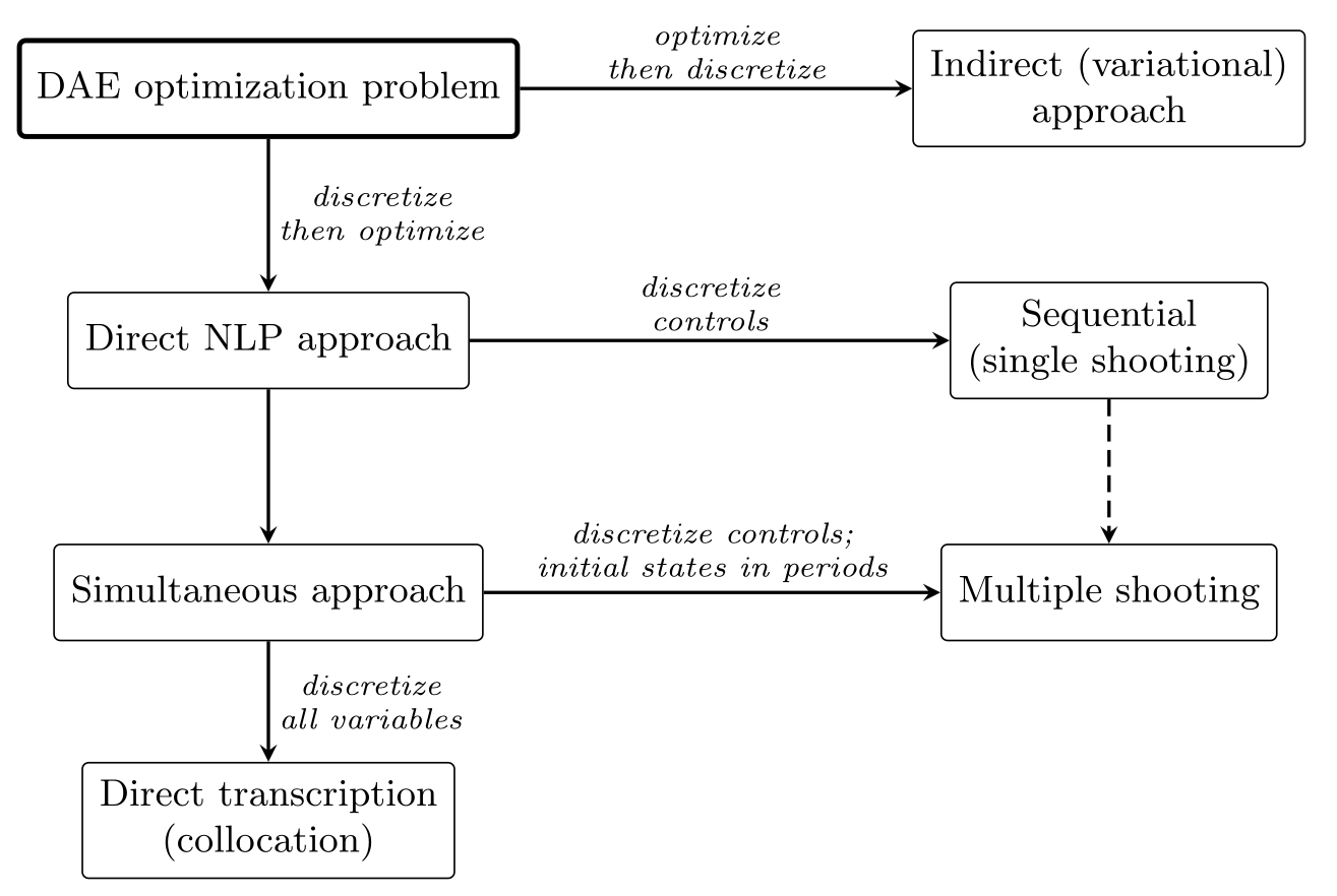
Classification of DAE optimization strategies

Re-authored as TikZ from Biegler (2010), Figure 8.10, p. 245; source at figures/tikz/dae-optimization-strategies.tex.

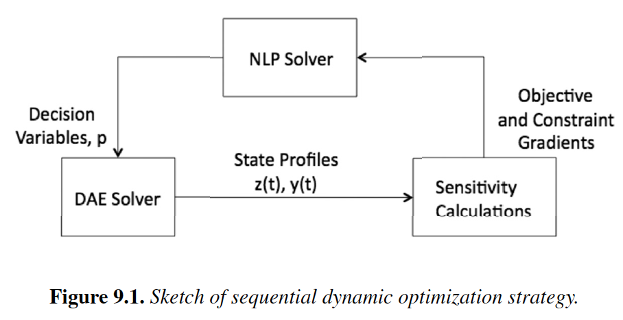
Chapter 9, Dynamic Optimization Methods with Embedded DAE Solvers: sequential and multiple-shooting methods.

Sequential dynamic optimization workflow with an optimizer repeatedly calling a DAE integrator

Chapter 10, Simultaneous Methods for Dynamic Optimization: direct collocation and large-scale NLP formulations.