Pyomo.DAE: Racing Example Revisited - Optimization for Decision Science

Prepared by: Prof. Alexander Dowling, Molly Dougher (mdoughe6@nd.edu, 2023)

# Install Pyomo and solvers for Google Colab
import sys

if "google.colab" in sys.modules:
    !wget "https://raw.githubusercontent.com/ndcbe/optimization/main/notebooks/helper.py"
    import helper

    helper.easy_install()
else:
    sys.path.insert(0, "../")
    import helper
helper.set_plotting_style()

# import Pyomo library
import pyomo.environ as pyo
import pyomo.dae as dae
import matplotlib.pyplot as plt
from pyomo.environ import units
from pyomo.util.check_units import assert_units_consistent

Car Example¶

Adapted from examples/dae/car_example.py

You are a race car driver with a simple goal. Drive distance $L$ in the minimal amount of time but come to a complete stop at the finish line.

Optimal Control Problem Formulation¶

Mathematically, you want to solve the following optimal control problem:

\begin{align*} \min_{u} \quad & t_f \\ \mathrm{s.t.} \quad & \frac{dx}{dt} = v \\ & \frac{dv}{dt} = u - R v^2 \\ & x(t=0) = 0, ~~ x(t=t_f) = L \\ & v(t=0) = 0, ~~ v(t=t_f) = 0 \\ & -3 \leq u \leq 1 \end{align*}

(1)

where $u$ is the acceleration/braking (your control variable) and $R$ is the drag coefficient (parameter).

Scale Time¶

Let $t = \tau \cdot t_f$ where $\tau \in [0,1]$ . Thus $dt = t_f d\tau$ . The optimal control problem becomes:

\begin{align*} \min_{u} \quad & t_f \\ \mathrm{s.t.} \quad & \frac{dx}{d\tau} = t_f v \\ & \frac{dv}{d\tau} = t_f (u - R v^2) \\ & x(\tau = 0) = 0, ~~ x(\tau = 1) = L \\ & v(\tau = 0) = 0, ~~ v(\tau = 1) = 0 \\ & -3 \leq u \leq 1 \end{align*}

(2)

Orthogonal Collocation on Finite Elements: Manual Approach¶

Here is the “classical”/“old school” way of manually implementing collocation on finite elements with sets.

Indices and Sets

Finite elements: $i \in \mathcal{I} = \{1,2,...,N_{FE}\}$
Finite elements (except first): $\mathcal{I} \setminus 1$
Internal collocation points: $j,k \in \mathcal{J} = \{1,2,...,N_{C}\}$

Parameters

Coefficients in collocation/Runge-Kutta formula: $a_{k,j}$
Drag coefficient: $R$
Race length: $L$
Scaled time for each finite element: $h_i = \frac{1}{N_{FE}}$

Variables

Position (internal collocation points): $x_{i,j}$
Position (beginning of each finite element): $\bar{x}_{i}$
Position derivative (internal collocation points): $\dot{x}_{i,j}$
Velocity (internal collocation points): $v_{i,j}$
Velocity (beginning of each finite element): $\bar{v}_{i}$
Velocity derivative (internal collocation points): $\dot{v}_{i,j}$
Time (internal collocation points): $t_{i,j}$
Time (beginning of each finite element): $\bar{t}_{i}$
Acceleration (control degrees of freedom): $u_i$

Objective and Constraints

\begin{align*} \min \quad & t_f \\ \mathrm{s.t.} \quad & \mathrm{Differential~equation~for~x:} \\ & x_{i,j} = \bar{x}_{i} + h_i \sum_{k \in \mathcal{J}} a_{k,j} \dot{x}_{i,k},\quad \forall i \in \mathcal{I},~j \in \mathcal{J} \\ & \bar{x}_{i} = \bar{x}_{i-1} + h_{i-1} \sum_{k \in \mathcal{J}} a_{k,N_C} \dot{x}_{i-1,k},\quad \forall i \in \mathcal{I} \setminus 1\\ & \dot{x}_{i,j} = t_f v_{i,j}, \quad \forall i \in \mathcal{I},~j \in \mathcal{J} \\ \\ & \mathrm{Differential~equation~for~v:} \\ & v_{i,j} = \bar{v}_{i} + h_i \sum_{k \in \mathcal{J}} a_{k,j} \dot{v}_{i,k},\quad \forall i \in \mathcal{I},~j \in \mathcal{J} \\ & \bar{v}_{i} = \bar{v}_{i-1} + h_{i-1} \sum_{k \in \mathcal{J}} a_{k,N_C} \dot{v}_{i-1,k},\quad \forall i \in \mathcal{I} \setminus 1\\ & \dot{v}_{i,j} = t_f (u_{i} - R v_{i,j}^2), \quad \forall i \in \mathcal{I},~j \in \mathcal{J} \\ \\ & \mathrm{Differential~equation~for~time:} \\ & t_{i,j} = \bar{t}_{i} + h_i \sum_{k \in \mathcal{J}} a_{k,j} t_f,\quad \forall i \in \mathcal{I},~j \in \mathcal{J} \\ & \bar{t}_{i} = \bar{t}_{i-1} + h_{i-1} \sum_{k \in \mathcal{J}} a_{k,N_C} t_f,\quad \forall i \in \mathcal{I} \setminus 1\\ \\ & \mathrm{Initial~conditions:} \\ & \bar{x}_{1} = 0, \quad \bar{v}_{1} = 0, \quad \bar{t}_1 = 0\\ \\ & \mathrm{Boundary~conditions:} \\ & L = \bar{x}_{N_{FE}} + h_{N_{FE}} \sum_{k \in \mathcal{J}} a_{k,N_C} \dot{x}_{N_{FE},k}, \\ & 0 = \bar{v}_{N_{FE}} + h_{N_{FE}} \sum_{k \in \mathcal{J}} a_{k,N_C} \dot{v}_{N_{FE},k}, \\ \\ & \mathrm{Bounds~on~acceleration:} \\ & -3 \leq u_i \leq 1, \quad \forall i \in \mathcal{I} \end{align*}

(3)

# Define the model
m2 = pyo.ConcreteModel()

# Define model parameters.
#
# R multiplies v**2 to give an acceleration, so R has units of 1/length.
m2.R = pyo.Param(initialize=0.001, units=1 / units.m)  # Friction factor
m2.L = pyo.Param(initialize=100.0, units=units.m)  # Final position

# Define finite elements and collocation points
NFE = 15  # Number of finite elements
NC = 3  # Number of collocation points
m2.I = pyo.Set(initialize=pyo.RangeSet(1, NFE))  # Set of finite elements
m2.J = pyo.Set(initialize=pyo.RangeSet(1, NC))  # Set of internal collocation points

# Define first order derivative collocation matrix
A = {}
A[1, 1] = 0.19681547722366
A[1, 2] = 0.39442431473909
A[1, 3] = 0.37640306270047
A[2, 1] = -0.06553542585020
A[2, 2] = 0.29207341166523
A[2, 3] = 0.51248582618842
A[3, 1] = 0.02377097434822
A[3, 2] = -0.04154875212600
A[3, 3] = 0.11111111111111

# Define A matrix as a model parameter (collocation coefficients are dimensionless)
m2.a = pyo.Param(m2.J, m2.J, initialize=A)

# Define step for each finite element. This is a fraction of the SCALED time
# tau in [0, 1], so it is dimensionless -- the physical step is h * tf seconds.
m2.h = pyo.Param(m2.I, initialize=1 / NFE)

# Define objective (final time)
m2.tf = pyo.Var(domain=pyo.NonNegativeReals, units=units.s)

# Variables for x (position). Because we differentiate with respect to the
# DIMENSIONLESS tau, xdot carries the same units as x itself.
m2.x0 = pyo.Var(m2.I, units=units.m)  # Beginning of each finite element
m2.x = pyo.Var(m2.I, m2.J, units=units.m)  # Internal collocation points
m2.xdot = pyo.Var(m2.I, m2.J, units=units.m)  # Derivative, internal collocation points

# Variables for v (velocity)
m2.v0 = pyo.Var(m2.I, units=units.m / units.s)  # Beginning of each finite element
m2.v = pyo.Var(m2.I, m2.J, units=units.m / units.s)  # Internal collocation points
m2.vdot = pyo.Var(
    m2.I, m2.J, units=units.m / units.s
)  # Derivative, internal collocation points

# Variables for t
m2.t0 = pyo.Var(m2.I, units=units.s)  # Beginning of each finite element
m2.t = pyo.Var(m2.I, m2.J, units=units.s)  # Internal collocation points

# Acceleration
m2.u = pyo.Var(
    m2.I, bounds=(-3, 1), units=units.m / units.s**2
)  # Control DOF (bounds in m/s**2)


### Finite Element Collocation Equations
# position
def FECOLx_(m2, i, j):
    return m2.x[i, j] == m2.x0[i] + m2.h[i] * sum(
        m2.a[k, j] * m2.xdot[i, k] for k in m2.J
    )


m2.FECOLx = pyo.Constraint(m2.I, m2.J, rule=FECOLx_)


# velocity
def FECOLv_(m2, i, j):
    return m2.v[i, j] == m2.v0[i] + m2.h[i] * sum(
        m2.a[k, j] * m2.vdot[i, k] for k in m2.J
    )


m2.FECOLv = pyo.Constraint(m2.I, m2.J, rule=FECOLv_)


# time
def FECOLt_(m2, i, j):
    return m2.t[i, j] == m2.t0[i] + m2.h[i] * sum(m2.a[k, j] * m2.tf for k in m2.J)


m2.FECOLt = pyo.Constraint(m2.I, m2.J, rule=FECOLt_)


### Continuity Equations
# position
def CONx_(m2, i):
    if i == 1:
        return pyo.Constraint.Skip
    else:
        return m2.x0[i] == m2.x0[i - 1] + m2.h[i - 1] * sum(
            m2.a[k, NC] * m2.xdot[i - 1, k] for k in m2.J
        )


m2.CONx = pyo.Constraint(m2.I, rule=CONx_)


# velocity
def CONv_(m2, i):
    if i == 1:
        return pyo.Constraint.Skip
    else:
        return m2.v0[i] == m2.v0[i - 1] + m2.h[i - 1] * sum(
            m2.a[k, NC] * m2.vdot[i - 1, k] for k in m2.J
        )


m2.CONv = pyo.Constraint(m2.I, rule=CONv_)


# time
def CONt_(m2, i):
    if i == 1:
        return pyo.Constraint.Skip
    else:
        return m2.t0[i] == m2.t0[i - 1] + m2.h[i - 1] * sum(
            m2.a[k, NC] * m2.tf for k in m2.J
        )


m2.CONt = pyo.Constraint(m2.I, rule=CONt_)


### Differential equations
# position
def ODEx_(m2, i, j):
    return m2.xdot[i, j] == m2.tf * m2.v[i, j]


m2.ODEx = pyo.Constraint(m2.I, m2.J, rule=ODEx_)


# velocity
def ODEv_(m2, i, j):
    return m2.vdot[i, j] == m2.tf * (m2.u[i] - m2.R * m2.v[i, j] ** 2)


m2.ODEv = pyo.Constraint(m2.I, m2.J, rule=ODEv_)

### Initial conditions
m2.xIC = pyo.Constraint(expr=m2.x0[1] == 0)
m2.vIC = pyo.Constraint(expr=m2.v0[1] == 0)
m2.tIC = pyo.Constraint(expr=m2.t0[1] == 0)

### Boundary conditions
m2.xBC = pyo.Constraint(
    expr=m2.L
    == m2.x0[NFE] + m2.h[NFE] * sum(m2.a[k, NC] * m2.xdot[NFE, k] for k in m2.J)
)
m2.vBC = pyo.Constraint(
    expr=0 == m2.v0[NFE] + m2.h[NFE] * sum(m2.a[k, NC] * m2.vdot[NFE, k] for k in m2.J)
)

### Set objective
m2.obj = pyo.Objective(expr=m2.tf)

### Check dimensional consistency.
#
# Here we wrote the collocation equations OURSELVES, so there is nothing for
# Pyomo to add later and nothing to trip over: the check works on the finished
# model. Compare with the Pyomo.dae version below, where the discretization
# equations are generated for us. See ./units_and_pyomo_dae.md
assert_units_consistent(m2)
print("Manual collocation model: units are consistent.")

Manual collocation model: units are consistent.

# Solve the model
solver = pyo.SolverFactory("ipopt")
results = solver.solve(m2, tee=True)
assert pyo.check_optimal_termination(results), (
    f"Solve failed: status={results.solver.status}, "
    f"termination={results.solver.termination_condition}"
)

print("final time = %6.2f" % (pyo.value(m2.tf)))

Ipopt 3.14.19: 

******************************************************************************
This program contains Ipopt, a library for large-scale nonlinear optimization.
 Ipopt is released as open source code under the Eclipse Public License (EPL).
         For more information visit https://github.com/coin-or/Ipopt
******************************************************************************

This is Ipopt version 3.14.19, running with linear solver MUMPS 5.8.2.

Number of nonzeros in equality constraint Jacobian...:     1093
Number of nonzeros in inequality constraint Jacobian.:        0
Number of nonzeros in Lagrangian Hessian.............:      105

Total number of variables............................:      286
                     variables with only lower bounds:        1
                variables with lower and upper bounds:       15
                     variables with only upper bounds:        0
Total number of equality constraints.................:      272
Total number of inequality constraints...............:        0
        inequality constraints with only lower bounds:        0
   inequality constraints with lower and upper bounds:        0
        inequality constraints with only upper bounds:        0

iter    objective    inf_pr   inf_du lg(mu)  ||d||  lg(rg) alpha_du alpha_pr  ls
   0  9.9999900e-03 1.00e+02 0.00e+00  -1.0 0.00e+00    -  0.00e+00 0.00e+00   0
   1r 9.9999900e-03 1.00e+02 9.99e+02   2.0 0.00e+00    -  0.00e+00 4.40e-08R  3
   2r 3.0578540e+00 9.99e+01 9.31e+02   2.0 4.49e+01    -  1.35e-01 6.80e-02f  2
   3r 2.2147899e+00 9.91e+01 5.68e+02   1.3 2.16e+00    -  1.00e+00 3.91e-01f  1
   4r 2.0632709e+00 9.88e+01 4.20e+02   0.6 1.92e+00    -  7.91e-01 2.59e-01f  1
   5r 2.8236279e+00 9.78e+01 2.47e+02   0.6 6.49e+00    -  5.25e-01 4.12e-01f  1
   6r 6.1897113e+00 9.47e+01 1.86e+02  -0.1 8.25e+00    -  3.79e-01 6.85e-01f  1
   7r 9.1974909e+00 8.83e+01 1.23e+02  -0.1 1.21e+01    -  2.99e-01 7.01e-01f  1
   8r 9.6970537e+00 8.58e+01 2.56e+00  -0.1 3.39e+00    -  1.00e+00 1.00e+00f  1
   9  9.9061474e+00 8.51e+01 9.92e-01  -1.0 1.15e+02    -  3.63e-01 7.81e-03h  8
iter    objective    inf_pr   inf_du lg(mu)  ||d||  lg(rg) alpha_du alpha_pr  ls
  10  1.0294740e+01 8.38e+01 1.07e+00  -1.0 1.17e+02    -  7.18e-01 1.56e-02h  7
  11  1.0567140e+01 8.26e+01 1.34e+00  -1.0 1.26e+02    -  6.33e-01 1.37e-02h  7
  12  1.0857928e+01 8.14e+01 1.50e+00  -1.0 1.27e+02    -  1.00e+00 1.55e-02h  7
  13  1.1129879e+01 8.01e+01 1.53e+00  -1.0 1.29e+02    -  6.12e-01 1.56e-02h  7
  14  1.1385223e+01 7.88e+01 1.53e+00  -1.0 1.28e+02    -  1.00e+00 1.56e-02h  7
  15  1.1622054e+01 7.76e+01 1.54e+00  -1.0 1.28e+02    -  7.40e-01 1.56e-02h  7
  16  1.1844930e+01 7.64e+01 1.52e+00  -1.0 1.27e+02    -  1.00e+00 1.56e-02h  7
  17  1.2052642e+01 7.52e+01 1.51e+00  -1.0 1.26e+02    -  8.77e-01 1.56e-02h  7
  18  1.2445299e+01 7.28e+01 1.45e+00  -1.0 1.25e+02    -  1.00e+00 3.12e-02h  6

  19  2.3532514e+01 7.88e+01 1.09e+00  -1.0 1.24e+02    -  1.00e+00 1.00e+00w  1
iter    objective    inf_pr   inf_du lg(mu)  ||d||  lg(rg) alpha_du alpha_pr  ls
  20  1.8234569e+01 3.92e+00 1.85e-01  -1.0 1.35e+01  -4.0 1.00e+00 1.00e+00w  1
  21  1.7447102e+01 6.62e-01 1.83e-02  -1.0 1.21e+01    -  1.00e+00 1.00e+00h  1
  22  1.6869098e+01 3.19e-01 3.70e-03  -1.7 3.77e+00    -  1.00e+00 1.00e+00h  1
  23  1.6787034e+01 2.38e-02 6.31e-05  -1.7 4.75e+00    -  1.00e+00 1.00e+00h  1
  24  1.6532561e+01 9.64e-02 3.22e-03  -3.8 3.50e+00    -  9.27e-01 1.00e+00h  1
  25  1.6522337e+01 3.01e-04 1.35e-06  -3.8 2.73e-01    -  1.00e+00 1.00e+00h  1
  26  1.6520217e+01 6.67e-06 3.99e-08  -5.7 2.72e-02    -  1.00e+00 1.00e+00h  1
  27  1.6520191e+01 1.13e-09 6.19e-12  -8.6 3.95e-04    -  1.00e+00 1.00e+00h  1

Number of Iterations....: 27

                                   (scaled)                 (unscaled)
Objective...............:   1.6520190872026856e+01    1.6520190872026856e+01
Dual infeasibility......:   6.1936299734013823e-12    6.1936299734013823e-12
Constraint violation....:   1.1293650459265336e-09    1.1293650459265336e-09
Variable bound violation:   2.1897113899882470e-08    2.1897113899882470e-08
Complementarity.........:   2.5313790462377002e-09    2.5313790462377002e-09
Overall NLP error.......:   2.5313790462377002e-09    2.5313790462377002e-09


Number of objective function evaluations             = 108
Number of objective gradient evaluations             = 22
Number of equality constraint evaluations            = 108
Number of inequality constraint evaluations          = 0
Number of equality constraint Jacobian evaluations   = 29
Number of inequality constraint Jacobian evaluations = 0
Number of Lagrangian Hessian evaluations             = 27
Total seconds in IPOPT                               = 0.209

EXIT: Optimal Solution Found.

final time =  16.52

Orthogonal Collocation on Finite Elements: Pyomo.dae¶

There is a better way! We can use Pyomo.dae to automatically formulate the collocation equations.

Declare Model¶

# Define the  model
m = pyo.ConcreteModel()

# Define the model parameters
m.R = pyo.Param(initialize=0.001, units=1 / units.m)  # Friction factor
m.L = pyo.Param(initialize=100.0, units=units.m)  # Final position

# Define time. The ContinuousSet cannot carry units -- it holds plain floats.
# Here that costs us nothing, because tau really IS dimensionless.
m.tau = dae.ContinuousSet(bounds=(0, 1))  # Dimensionless (scaled) time
m.time = pyo.Var(m.tau, units=units.s)  # Physical time
m.tf = pyo.Var(units=units.s)  # Final time

# Define remaining algebraic variables
m.x = pyo.Var(m.tau, bounds=(0, m.L + 50 * units.m), units=units.m)  # Position
m.v = pyo.Var(m.tau, bounds=(0, None), units=units.m / units.s)  # Velocity
m.u = pyo.Var(
    m.tau, bounds=(-3.0, 1.0), initialize=0, units=units.m / units.s**2
)  # Acceleration

# Define derivative variables.
#
# DerivativeVar defaults to DIMENSIONLESS -- it does not inherit units from the
# state variable. And because tau is dimensionless, d/dtau carries the SAME
# units as the state, not the state's units per second.
m.dtime = dae.DerivativeVar(m.time, units=units.s)
m.dx = dae.DerivativeVar(m.x, units=units.m)
m.dv = dae.DerivativeVar(m.v, units=units.m / units.s)

# Declare the objective (minimize final time)
m.obj = pyo.Objective(expr=m.tf)


# Define the constraints
# position
def _ode1(m, i):
    if i == 0:
        return pyo.Constraint.Skip
    return m.dx[i] == m.tf * m.v[i]


m.ode1 = pyo.Constraint(m.tau, rule=_ode1)


# velocity
def _ode2(m, i):
    if i == 0:
        return pyo.Constraint.Skip
    return m.dv[i] == m.tf * (m.u[i] - m.R * m.v[i] ** 2)


m.ode2 = pyo.Constraint(m.tau, rule=_ode2)


# time
def _ode3(m, i):
    if i == 0:
        return pyo.Constraint.Skip
    return m.dtime[i] == m.tf


m.ode3 = pyo.Constraint(m.tau, rule=_ode3)


# Define the inital/boundary conditions
def _init(m):
    yield m.x[0] == 0
    yield m.x[1] == m.L
    yield m.v[0] == 0
    yield m.v[1] == 0
    yield m.time[0] == 0


m.initcon = pyo.ConstraintList(rule=_init)

# Check units NOW, before the next cell discretizes the model.
# See ./units_and_pyomo_dae.md and https://github.com/Pyomo/pyomo/issues/1790
assert_units_consistent(m)
print("Pyomo.dae model: units are consistent (before discretization).")

Pyomo.dae model: units are consistent (before discretization).

Discretize/Transcribe and Solve¶

# discretizer = TransformationFactory('dae.finite_difference')
# discretizer.apply_to(m,nfe=15,scheme='BACKWARD')

# Declare the discretizer
discretizer = pyo.TransformationFactory("dae.collocation")
discretizer.apply_to(m, nfe=15, scheme="LAGRANGE-RADAU", ncp=3)
# discretizer.apply_to(m,nfe=15,scheme='LAGRANGE-LEGENDRE',ncp=3)

# force piecewise constant controls (acceleration) over each finite element
m = discretizer.reduce_collocation_points(m, var=m.u, ncp=1, contset=m.tau)

# Solve
solver = pyo.SolverFactory("ipopt")
results = solver.solve(m, tee=True)
assert pyo.check_optimal_termination(results), (
    f"Solve failed: status={results.solver.status}, "
    f"termination={results.solver.termination_condition}"
)

print("final time = %6.2f" % (pyo.value(m.tf)))

Ipopt 3.14.19: 

******************************************************************************
This program contains Ipopt, a library for large-scale nonlinear optimization.
 Ipopt is released as open source code under the Eclipse Public License (EPL).
         For more information visit https://github.com/coin-or/Ipopt
******************************************************************************

This is Ipopt version 3.14.19, running with linear solver MUMPS 5.8.2.

Number of nonzeros in equality constraint Jacobian...:     1145
Number of nonzeros in inequality constraint Jacobian.:        0
Number of nonzeros in Lagrangian Hessian.............:      135

Total number of variables............................:      319
                     variables with only lower bounds:       46
                variables with lower and upper bounds:       91
                     variables with only upper bounds:        0
Total number of equality constraints.................:      305
Total number of inequality constraints...............:        0
        inequality constraints with only lower bounds:        0
   inequality constraints with lower and upper bounds:        0
        inequality constraints with only upper bounds:        0

iter    objective    inf_pr   inf_du lg(mu)  ||d||  lg(rg) alpha_du alpha_pr  ls
   0  0.0000000e+00 1.00e+02 1.90e-11  -1.0 0.00e+00    -  0.00e+00 0.00e+00   0
   1  2.6778732e+00 1.00e+02 1.45e+10  -1.0 1.00e+04    -  9.91e-05 2.68e-04f  2
   2  2.7435398e+00 9.92e+01 2.02e+11  -1.0 2.35e+02  10.0 1.82e-04 7.48e-03f  1

   3  2.7602544e+00 9.92e+01 2.02e+11  -1.0 1.95e+02   9.5 7.91e-03 1.96e-04h  1

   4r 2.7602544e+00 9.92e+01 9.99e+02   2.0 0.00e+00   9.0 0.00e+00 3.53e-07R  4
   5r 2.5779677e+00 9.87e+01 9.76e+02   2.0 1.58e+02    -  2.13e-02 2.35e-02f  1
   6r 2.5483326e+00 9.87e+01 9.32e+02   0.6 1.97e+01    -  3.10e-01 4.48e-02f  1
   7r 4.8140117e+00 9.72e+01 6.16e+02   0.6 7.43e+00    -  3.24e-01 3.39e-01f  1
   8r 7.2317323e+00 9.36e+01 2.39e+02   0.6 9.57e+00    -  8.05e-01 6.12e-01f  1
   9r 7.8296215e+00 9.13e+01 4.03e+00   0.6 3.05e+00    -  1.00e+00 1.00e+00f  1
iter    objective    inf_pr   inf_du lg(mu)  ||d||  lg(rg) alpha_du alpha_pr  ls
  10r 7.7888770e+00 9.15e+01 1.91e+01  -1.5 3.87e-01    -  9.83e-01 7.05e-01f  1
  11r 1.2026369e+01 8.67e+01 3.31e+01  -1.5 1.51e+03    -  8.76e-03 1.14e-02f  1

  12  6.7694748e+00 7.12e+01 1.53e+01  -1.0 2.14e+02    -  8.96e-02 1.78e-01H  1
  13  1.3562972e+01 6.40e+01 3.55e+01  -1.0 2.03e+02    -  4.91e-03 1.02e-01h  4
  14  1.4595495e+01 6.25e+01 3.97e+00  -1.0 1.82e+02    -  1.77e-01 2.29e-02h  3
  15  1.5360918e+01 6.14e+01 3.90e+00  -1.0 2.05e+02    -  1.58e-02 1.69e-02h  3

  16  1.5444142e+01 6.10e+01 2.20e+08  -1.0 7.85e+01   8.6 4.32e-02 7.58e-03h  2
  17  1.5490295e+01 6.07e+01 2.59e+08  -1.0 7.80e+01   8.1 9.02e-02 4.13e-03h  2
  18  1.5545183e+01 6.04e+01 2.73e+08  -1.0 7.77e+01   7.6 1.24e-01 4.67e-03h  1
  19  1.5546018e+01 6.04e+01 2.73e+08  -1.0 7.75e+01   7.1 1.80e-01 6.26e-05h  1
iter    objective    inf_pr   inf_du lg(mu)  ||d||  lg(rg) alpha_du alpha_pr  ls
  20  1.5591528e+01 6.03e+01 2.73e+08  -1.0 8.12e+01   6.7 9.55e-02 2.46e-03h  1
  21  1.5763195e+01 6.00e+01 4.03e+08  -1.0 1.47e+02   6.2 4.20e-01 5.37e-03h  1
  22  1.5765409e+01 6.00e+01 4.98e+08  -1.0 8.32e+01   6.6 8.36e-02 1.17e-04h  1

  23  1.6488242e+01 5.87e+01 5.99e+09  -1.0 1.71e+02   6.1 7.80e-01 2.04e-02h  1
  24  2.5858192e+01 2.99e+01 1.22e+09  -1.0 8.55e+01   6.6 9.92e-02 4.92e-01h  1
  25  3.1055324e+01 6.06e+00 1.77e+09  -1.0 5.20e+01   6.1 5.46e-01 9.90e-01h  1
  26  3.0700300e+01 8.44e-02 3.59e+08  -1.0 1.68e+00   5.6 9.32e-01 9.90e-01h  1
  27  3.0695155e+01 8.06e-06 1.36e+08  -1.0 2.21e-02   5.1 3.13e-01 1.00e+00h  1

  28  3.0695155e+01 1.63e-12 8.18e+07  -1.0 2.35e-06   4.6 7.05e-01 1.00e+00f  1

  29  2.7369752e+01 3.89e+00 8.08e+07  -1.0 1.64e+03    -  6.05e-02 2.51e-02f  1
iter    objective    inf_pr   inf_du lg(mu)  ||d||  lg(rg) alpha_du alpha_pr  ls
  30  2.4498338e+01 7.09e+00 7.52e+07  -1.0 3.30e+02    -  2.84e-01 1.18e-01f  2
  31  1.9942276e+01 1.49e+01 4.80e+07  -1.0 1.30e+02    -  6.35e-01 3.60e-01h  1
  32  1.9783577e+01 1.19e+00 1.45e+07  -1.0 5.63e+01    -  4.49e-01 9.14e-01h  1
  33  1.8715151e+01 2.88e+00 2.96e+06  -1.0 4.91e+01    -  6.26e-01 9.79e-01f  1
  34  1.8939163e+01 9.96e-02 2.69e+06  -1.0 9.56e+00    -  5.15e-01 1.00e+00f  1

  35  1.8890595e+01 1.05e-02 5.09e+05  -1.0 3.88e+00    -  6.57e-01 1.00e+00h  1
  36  1.8898687e+01 3.23e-04 4.54e+05  -1.0 7.31e-01    -  5.10e-01 1.00e+00f  1
  37  1.8898221e+01 1.22e-06 8.53e+04  -1.0 4.66e-02    -  6.57e-01 1.00e+00f  1
  38  1.8898301e+01 1.56e-08 7.62e+04  -1.0 3.35e-03    -  5.10e-01 1.00e+00f  1
  39  1.8898433e+01 7.65e-09 1.45e+04  -1.0 7.02e-04   4.2 6.54e-01 1.00e+00f  1
iter    objective    inf_pr   inf_du lg(mu)  ||d||  lg(rg) alpha_du alpha_pr  ls
  40  1.8898817e+01 1.04e-04 1.23e+04  -1.0 2.89e-03   3.7 2.12e-01 1.00e+00f  1
  41  1.8898884e+01 7.79e-05 9.91e+03  -1.0 3.31e-03   3.2 7.74e-01 2.50e-01f  3
  42  1.8900091e+01 2.82e-05 2.95e+03  -1.0 4.93e-03   2.7 2.66e-01 1.00e+00f  1

  43  1.8901390e+01 2.34e-05 1.99e+02  -1.0 6.21e-03   2.3 8.50e-01 1.00e+00f  1
  44  1.8901444e+01 2.13e-09 1.16e+05  -2.5 6.92e-04   1.8 9.88e-01 1.00e+00h  1
  45  1.8902191e+01 2.21e-07 8.53e-02  -2.5 4.18e-03   1.3 1.00e+00 1.00e+00f  1
  46  1.8901379e+01 2.99e-07 5.98e-01  -3.8 2.16e-03   0.8 1.00e+00 1.00e+00h  1

  47  1.8895298e+01 1.69e-05 1.39e-02  -3.8 1.84e-02  -0.1 1.00e+00 1.00e+00f  1
  48  1.8872254e+01 2.67e-04 1.51e-02  -3.8 1.80e-01  -1.1 1.00e+00 1.00e+00h  1
  49  1.8660674e+01 2.25e-02 1.49e-02  -3.8 1.60e+00  -2.0 1.00e+00 1.00e+00f  1

iter    objective    inf_pr   inf_du lg(mu)  ||d||  lg(rg) alpha_du alpha_pr  ls
  50  1.8265078e+01 8.91e-02 1.32e-01  -3.8 4.68e+00  -2.5 1.00e+00 6.31e-01h  1
  51  1.7969301e+01 1.33e-01 5.59e-01  -3.8 2.88e+01  -3.5 1.00e+00 7.53e-02h  1
  52  1.7709695e+01 1.66e-01 7.68e-01  -3.8 2.16e+01  -3.5 1.00e+00 9.44e-02h  1

  53  1.7471956e+01 1.89e-01 8.40e-01  -3.8 1.69e+01  -3.6 1.00e+00 1.33e-01h  1
  54  1.7121513e+01 3.28e-01 9.55e-01  -3.8 7.33e+01  -4.5 5.00e-01 5.87e-02h  1

  55  1.6965032e+01 3.76e-01 6.29e-01  -3.8 1.25e+02  -4.6 1.00e+00 5.55e-02h  1
  56  1.6785245e+01 5.95e-01 6.23e-01  -3.8 3.42e+03    -  8.87e-03 6.32e-03f  1
  57  1.6694793e+01 6.04e-01 7.91e-01  -3.8 1.85e+02    -  4.15e-01 2.23e-02h  1
  58  1.6559174e+01 3.60e-01 4.73e-01  -3.8 2.71e+01    -  4.61e-01 4.09e-01h  1

  59  1.6529962e+01 1.15e-01 1.62e-01  -3.8 2.54e+00    -  1.00e+00 6.81e-01h  1
iter    objective    inf_pr   inf_du lg(mu)  ||d||  lg(rg) alpha_du alpha_pr  ls
  60  1.6526420e+01 1.29e-04 1.13e+00  -3.8 5.56e-01    -  8.98e-02 1.00e+00h  1
  61  1.6526503e+01 2.67e-08 1.51e-09  -3.8 5.22e-03    -  1.00e+00 1.00e+00h  1
  62  1.6520275e+01 6.32e-05 1.05e-06  -5.7 9.59e-02    -  1.00e+00 1.00e+00f  1
  63  1.6520269e+01 7.57e-11 1.04e+06  -5.7 1.32e-04    -  1.42e-02 1.00e+00h  1
  64  1.6520269e+01 1.39e-12 2.43e-10  -5.7 4.14e-09    -  1.00e+00 1.00e+00h  1
  65  1.6520192e+01 9.76e-09 1.62e-10  -8.6 1.19e-03    -  1.00e+00 1.00e+00f  1

Number of Iterations....: 65

                                   (scaled)                 (unscaled)
Objective...............:   1.6520191521080921e+01    1.6520191521080921e+01
Dual infeasibility......:   1.6218770571595899e-10    1.6218770571595899e-10
Constraint violation....:   9.7603845006233314e-09    9.7603845006233314e-09
Variable bound violation:   5.4130766535820385e-09    5.4130766535820385e-09
Complementarity.........:   2.5852537826788002e-09    2.5852537826788002e-09
Overall NLP error.......:   9.7603845006233314e-09    9.7603845006233314e-09


Number of objective function evaluations             = 89
Number of objective gradient evaluations             = 60
Number of equality constraint evaluations            = 89
Number of inequality constraint evaluations          = 0
Number of equality constraint Jacobian evaluations   = 67
Number of inequality constraint Jacobian evaluations = 0
Number of Lagrangian Hessian evaluations             = 65
Total seconds in IPOPT                               = 0.937

EXIT: Optimal Solution Found.

final time =  16.52

Plot Results¶

# Define empty lists
x = []  # position, units of length
v = []  # velocity, units of length per time
u = []  # acceleration, units of length per time squared
time = []  # time

# Loop over time and append the solution values for each variable to their respective lists
for i in m.tau:
    time.append(pyo.value(m.time[i]))
    x.append(pyo.value(m.x[i]))
    v.append(pyo.value(m.v[i]))
    u.append(pyo.value(m.u[i]))

# Make a figure
plt.figure(figsize=(12, 4))

# Format subplot 1 (position)
plt.subplot(131)
plt.plot(time, x, linewidth=3, label="x")
plt.title("location (m)", fontsize=16, fontweight="bold")
plt.xlabel("time (s)", fontsize=16, fontweight="bold")
plt.tick_params(direction="in", labelsize=15)

# Format subplot 2 (velocity)
plt.subplot(132)
plt.plot(time, v, linewidth=3, label="v")
plt.xlabel("time (s)", fontsize=16, fontweight="bold")
plt.title("velocity (m/s)", fontsize=16, fontweight="bold")
plt.tick_params(direction="in", labelsize=15)

# Format subplot 3 (acceleration)
plt.subplot(133)
plt.plot(time, u, linewidth=3, label="u")
plt.xlabel("time (s)", fontsize=16, fontweight="bold")
plt.title("acceleration (m/s$^2$)", fontsize=16, fontweight="bold")
plt.tick_params(direction="in", labelsize=15)

plt.show()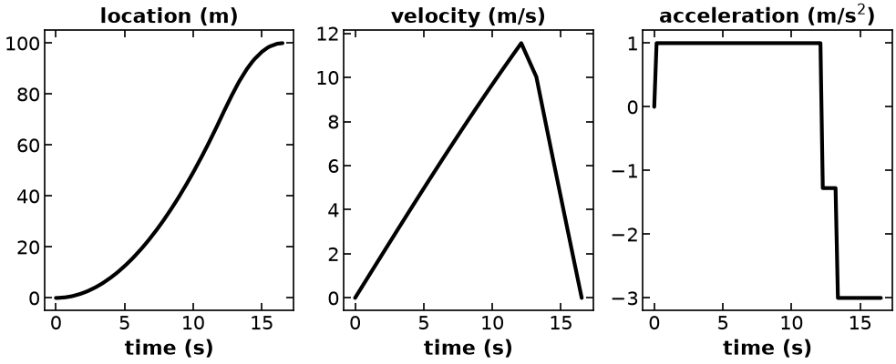

Discussion Questions

How does the time/number of evaluations that IPOPT needs to solve the problem change for a discretized versus non-discretized model?
Check to make sure that these results make sense. Based on the known derivative relationships between position, velocity, and acceleration, do the 3 plots make sense? Hint: Match up the trends in each graph.