This page is adapted from our process control class at Notre Dame; it was developed by Prof. Jeff Kantor.
Source material.
Jeffrey Kantor. Open-Loop Optimal Control, in CBE 30338 Data Analytics, Optimization, and Control at the University of Notre Dame,
notebooks/6/Simulation-and-Open-Loop-Optimal-Control.ipynb. Most of that course’s material was developed by Prof. Kantor, who passed away in 2023.
Alexander W. Dowling, Molly Dougher, Madelynn J. Watson, Hailey G. Lynch, Zhicheng Lu, and Daniel J. Laky (2025). Teaching Digital Twins in Process Control Using the Temperature Control Lab. ESCAPE 35 – European Symposium on Computer Aided Process Engineering, Ghent, Belgium, 6–9 July 2025. Ed. by Jan F. M. Van Impe, Grégoire Léonard, Satyajeet S. Bhonsale, Monika E. Polańska, and Filip Logist. Peer-reviewed conference proceeding, Systems and Control Transactions, Vol. 4, p. 2215 – 2221. Dowling et al. (2025)
The conference paper describes the TCLab-based redesign of that process control course, not this one; the two-state heater/sensor model used below appears there as Eqs. (3)–(4).
Learning Objectives
Review syntax for Pyomo.DAE
See how an optimization problem with zero degrees of freedom is a simulation problem
Practice using the units feature in Pyomo
See why a units-correct
Pyomo.daemodel must be checked before discretization (see Units in Pyomo.dae Models)
Install Packages and Load Modules
# Install Pyomo and solvers for Google Colab
import sys

if "google.colab" in sys.modules:
    !wget "https://raw.githubusercontent.com/ndcbe/optimization/main/notebooks/helper.py"
    import helper

    helper.easy_install()
else:
    sys.path.insert(0, "../")
    import helper
helper.set_plotting_style()

# import Pyomo library
import pyomo.environ as pyo
import pyomo.dae as dae
import matplotlib.pyplot as plt
from pyomo.environ import units
from pyomo.util.check_units import assert_units_consistent
Temperature Control Lab Dynamic Model
The temperature control lab is an Arduino-based hands-on experiment for teaching dynamic modeling and process control developed by Prof. John Hedengren. At Notre Dame, we restructured our core undergraduate process control class around six hands-on laboratory assignments with the TCLab.
The TCLab board contains two heater plus temperature sensor assemblies. Using Python (or MATLAB), students can independently manipulate the electrical power to the heaters and measure the temperatures.
For simplicity, we will develop a mathematical single heater and temperature sensor assembly. However, this workshop example also supports modeling both assemblies.
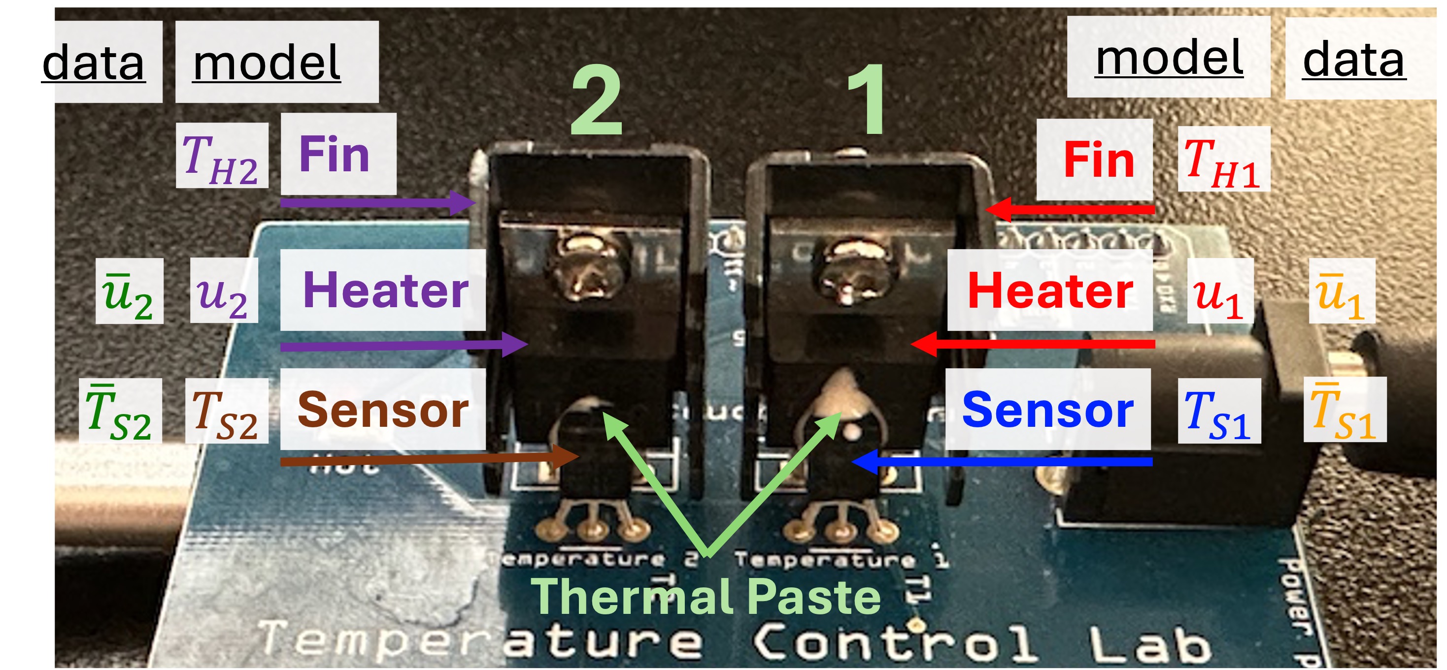
We will define two states:
is the temperature of the heater/fin assembly (°C)
is the temperature of the sensor (°C)
Assumptions:
The two bodies are uniform temperature, i.e., we are neglecting any temperature gradients in the fin.
The sensor exchanges heat only with the heater, and heat transfer to the surroundings is dominated by the heat sink attached to the heater.
Heat capacities are constant.
Radiative heat transfer is negligible.
We define the manipulated variable:
is the power sent to the heater (% of max)
This motivates the following model:
The model has the following unknown parameters:
is the heat capacity of the heater/fin assembly (J / °C)
is the heat capacity of the sensor (J / °C)
is the heat transfer coefficient from the heater/fin to ambient (W / °C)
is the heat transfer coefficient from the heater/fin to the sensor (W / °C)
And the following known parameters:
are constants for the TCLab (W / %)
is the ambient temperature (°C)
Let’s start by defining some model coefficients:
# parameters
# alpha * P converts heater command (%) to power (W), so alpha*P must be W / %.
# Percent is dimensionless, so W / % is just W.
alpha = 0.00016 * units.W  # W per (unit of P * percent of u1)
P = 200  # dimensionless scale factor for the heater
Ua = (
    0.050 * units.W / units.kelvin
)  # heat transfer coefficient from heater to environment
CpH = 2.2 * units.J / units.kelvin  # heat capacity of the heater (J/deg C)
CpS = 1.9 * units.J / units.kelvin  # heat capacity of the sensor (J/deg C)
Ub = 0.021 * units.W / units.kelvin  # heat transfer coefficient from heater to sensor
Tamb_C = 21.0  # ambient temperature in deg C
Tamb = units.convert_temp_C_to_K(Tamb_C) * units.kelvin  # ambient temperature
Simulate a Step Test (ramp)
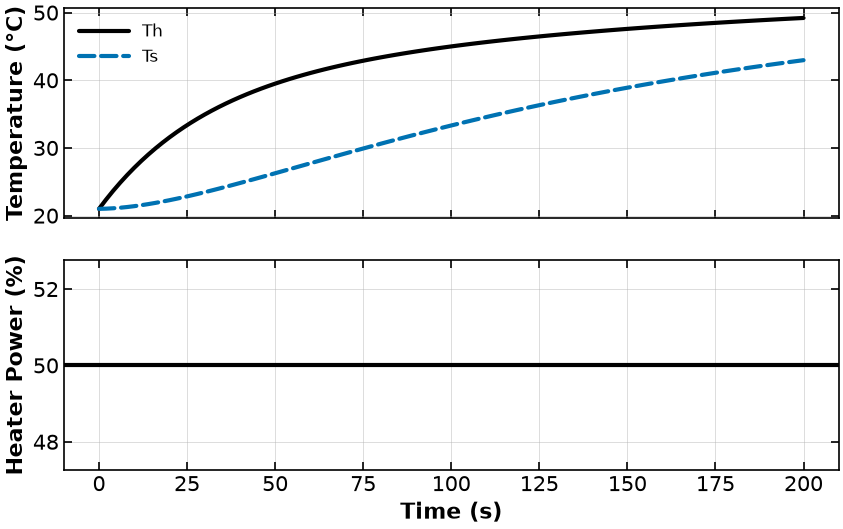
We will start by simulating our TCLab model. In other words, we will solve the following optimization problem with zero degrees of freedom:
Here “s.t.” means “subject to”, i.e., the constraints.
# Final time [seconds].
#
# Why no units here? A ContinuousSet cannot carry units. This is Pyomo issue
# #1790, still open: https://github.com/Pyomo/pyomo/issues/1790
# It is also the reason we must check units BEFORE discretizing -- see the
# section below and ./units_and_pyomo_dae.md
tf = 200

# control input [%]
u = 50.0

# Create a Pyomo model
m = pyo.ConcreteModel("TCLab Heater/Sensor")

# Define time domain
m.t = dae.ContinuousSet(bounds=(0, tf))

# Define the state variables as a function of time
m.Th = pyo.Var(m.t, units=units.kelvin)
m.Ts = pyo.Var(m.t, units=units.kelvin)

# Define the derivatives of the state variables.
#
# DerivativeVar defaults to DIMENSIONLESS -- it does not inherit units from the
# state variable. Here m.t is time in seconds, so dT/dt is K/s. Say it explicitly.
m.dTh = dae.DerivativeVar(m.Th, units=units.kelvin / units.s)
m.dTs = dae.DerivativeVar(m.Ts, units=units.kelvin / units.s)


# Define the first differential equation
@m.Constraint(m.t)
def heater1(m, t):
    return (
        CpH * m.dTh[t]
        == Ua * (Tamb - m.Th[t]) + Ub * (m.Ts[t] - m.Th[t]) + alpha * P * u
    )


# Define the second differential equation
@m.Constraint(m.t)
def sensor1(m, t):
    return CpS * m.dTs[t] == Ub * (m.Th[t] - m.Ts[t])


# Set the initial conditions
m.Th[0].fix(Tamb)
m.Ts[0].fix(Tamb)

# Check dimensional consistency NOW, while the model is still continuous.
# After discretization this same call raises InconsistentUnitsError -- see below.
assert_units_consistent(m)
print("Units are consistent (continuous model, before discretization).")

# Apply a finite difference formula to numerically integrate the differential equations
pyo.TransformationFactory("dae.finite_difference").apply_to(m, nfe=100, wrt=m.t)

# Call our nonlinear optimization/equation solver, Ipopt
results = pyo.SolverFactory("ipopt").solve(m)
assert pyo.check_optimal_termination(results), (
    f"Solve failed: status={results.solver.status}, "
    f"termination={results.solver.termination_condition}"
)

# Plot the results
fig, ax = plt.subplots(2, 1, figsize=(10, 6), sharex=True)

# Plot 1: Temperature
ax[0].plot(m.t, [units.convert_temp_K_to_C(m.Th[t]()) for t in m.t], label="Th")
ax[0].plot(
    m.t, [units.convert_temp_K_to_C(m.Ts[t]()) for t in m.t], label="Ts", linestyle="--"
)
ax[0].legend()
ax[0].set_ylabel("Temperature (°C)")
ax[0].grid()

# Plot 2: Heater Power
ax[1].axhline(u, label="Power")
ax[1].set_xlabel("Time (s)")
ax[1].set_ylabel("Heater Power (%)")
ax[1].grid()
plt.show()
Units are consistent (continuous model, before discretization).
Why the units check comes before TransformationFactory
The cell above called assert_units_consistent(m) immediately before discretizing.
The order is not cosmetic.
Here is what happened. A backward difference for at time is
and Pyomo writes it out with already evaluated to a number:
dTh[2.0] == 0.5*(Th[2.0] - Th[0])That 0.5 is , and it should carry units of .
It does not. A ContinuousSet stores plain Python floats and cannot hold units, which
is exactly why tf = 200 above has its units only in a comment. Pyomo therefore reads
the right-hand side as a temperature and the left-hand side as a temperature rate,
and reports -- correctly, given what it can see -- that they disagree.
This is Pyomo issue #1790, still open. Nothing is wrong with our model and nothing is wrong with the finite-difference arithmetic; the units container simply has nowhere to record what the time domain is measured in.
The practical rule is short:
Declare units on everything, then
assert_units_consistentat the end of your model-building function, before any discretization.
You give up nothing by checking early. The discretization equations are generated by Pyomo, not written by you, so they are not where your modeling errors hide. Checking the continuous model checks every equation you actually typed.
Run the cell below to see the failure for yourself.
# Reproduce the failure. The model `m` above has already been discretized, so
# asserting on it now raises -- even though the SAME model passed the check moments
# before `TransformationFactory` was applied.

try:
    assert_units_consistent(m)
    print("Units are consistent -- unexpected!")
except Exception as e:
    print(type(e).__name__)
    print(e)
ERROR: Units problem with expression dTh[2.0] - 0.5*(Th[2.0] - Th[0])
ERROR: Error in units when checking dTh_disc_eq[2.0]
InconsistentUnitsError
Error in units found in expression: dTh[2.0] - 0.5*(Th[2.0] - Th[0]): kelvin / second not compatible with kelvin.
The code below to access and print results from the Pyomo model:
for i, t in enumerate(m.t):
    # Only print every 10 timesteps
    if i % 10 == 0:
        print(
            "Th=",
            round(pyo.value(m.Th[t]), 2),
            "K and Ts=",
            round(pyo.value(m.Ts[t]), 2),
            "K at time",
            round(t, 2),
            "seconds.",
        )
Th= 294.15 K and Ts= 294.15 K at time 0 seconds.
Th= 304.71 K and Ts= 295.43 K at time 20.0 seconds.
Th= 310.66 K and Ts= 297.97 K at time 40.0 seconds.
Th= 314.23 K and Ts= 300.88 K at time 60.0 seconds.
Th= 316.54 K and Ts= 303.78 K at time 80.0 seconds.
Th= 318.16 K and Ts= 306.47 K at time 100.0 seconds.
Th= 319.37 K and Ts= 308.91 K at time 120.0 seconds.
Th= 320.33 K and Ts= 311.07 K at time 140.0 seconds.
Th= 321.12 K and Ts= 312.98 K at time 160.0 seconds.
Th= 321.79 K and Ts= 314.66 K at time 180.0 seconds.
Th= 322.36 K and Ts= 316.12 K at time 200 seconds.
Uncomment and run the code below to see the details of the Pyomo model:
# m.pprint()Activity: Optimization by Trial-and-Error
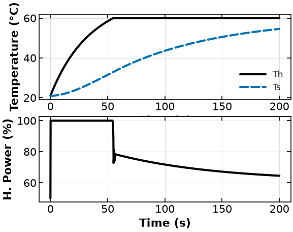
Modify the code above to find the value for u that causes Th to reach 60 °C at the final time. In others words, we are using trial and error to solve the following optimization problem:
Feedforward Optimal Control
An optimal control policy minimizes the differences
subject to constraints
This is different than our example above because we allow to have a unique value for each timestep.
Note that pyomo.dae has an Integral object to help with these situations.
# Set point, deg C
SP = units.convert_temp_C_to_K(60.0) * units.kelvin

# Create a Pyomo model
m = pyo.ConcreteModel("TCLab Heater/Sensor")

# Define time domain
m.t = dae.ContinuousSet(bounds=(0, tf))

# Define the state variables as a function of time
m.Th = pyo.Var(m.t, units=units.kelvin)
m.Ts = pyo.Var(m.t, units=units.kelvin)

# Define the derivatives of the state variables (K/s -- state it explicitly)
m.dTh = dae.DerivativeVar(m.Th, units=units.kelvin / units.s)
m.dTs = dae.DerivativeVar(m.Ts, units=units.kelvin / units.s)

# Define the control variable (heater power, % of max) as a function of time.
# Percent is dimensionless; alpha * P carries the W / % conversion.
m.u = pyo.Var(m.t, bounds=(0, 100))


# Define the integral of the squared error
@m.Integral(m.t)
def ise(m, t):
    return (SP - m.Th[t]) ** 2


# Define the first differential equation
# Notice we are defining the equation using the decorator syntax
@m.Constraint(m.t)
def heater1(m, t):
    return (
        CpH * m.dTh[t]
        == Ua * (Tamb - m.Th[t]) + Ub * (m.Ts[t] - m.Th[t]) + alpha * P * m.u[t]
    )


# Define the second differential equation
@m.Constraint(m.t)
def sensor1(m, t):
    return CpS * m.dTs[t] == Ub * (m.Th[t] - m.Ts[t])


# Set the initial conditions
m.Th[0].fix(Tamb)
m.Ts[0].fix(Tamb)


# Define the objective function
@m.Objective(sense=pyo.minimize)
def objective(m):
    return m.ise


# Units, again checked on the continuous model before discretizing.
#
# Note that m.ise comes out in K**2, not K**2 * s. pyomo.dae builds the Integral
# as a weighted sum whose quadrature weights are dimensionless -- the same
# consequence of issue #1790. The objective is still internally consistent, so
# the check passes.
assert_units_consistent(m)
print("ise units:", units.get_units(m.ise))

# Apply a collocation method to numerically integrate the differential equations
pyo.TransformationFactory("dae.collocation").apply_to(m, nfe=200, wrt=m.t)

# Call our nonlinear optimization/equation solver, Ipopt
results = pyo.SolverFactory("ipopt").solve(m)
assert pyo.check_optimal_termination(results), (
    f"Solve failed: status={results.solver.status}, "
    f"termination={results.solver.termination_condition}"
)


# We are going to repeat plotting two more times,
# so let's define a function
def plot_results(m):
    """
    Plot results from Pyomo optimization

    Arguments:
    m: Pyomo model

    Returns:
    Nothing

    """

    # Plot the results
    fig, ax = plt.subplots(2, 1)

    ax[0].plot(m.t, [units.convert_temp_K_to_C(m.Th[t]()) for t in m.t], label="Th")
    ax[0].plot(
        m.t,
        [units.convert_temp_K_to_C(m.Ts[t]()) for t in m.t],
        label="Ts",
        linestyle="--",
    )
    ax[0].legend()
    ax[0].set_xlabel("Time (s)")
    ax[0].set_ylabel("Temperature (°C)")
    ax[0].grid()

    ax[1].plot(m.t, [m.u[t]() for t in m.t], label="u")
    ax[1].set_xlabel("Time (s)")
    ax[1].set_ylabel("H. Power (%)")
    ax[1].grid()


plot_results(m)
ise units: K**2
Controlling to a Reference Trajectory
Now let’s consider optimizing the control input to track a more sophisticated time-varying setpoint signal .
Python function r(t) uses numpy.interp to compute values of the reference trajectory at any point in time.
import numpy as np

# time grid
tf = 1000
dt = 2
n = round(tf / dt)
t_grid = np.linspace(0, tf, n + 1)


# setpoint/reference
def r(t):
    return np.interp(t, [0, 50, 150, 450, 550], [Tamb_C, Tamb_C, 60, 60, 35])


# plot function
fig, ax = plt.subplots(1, 1, figsize=(10, 3))
ax.plot(t_grid, r(t_grid), label="setpoint")
ax.set_title("setpoint")
ax.set_ylabel("Temperature (°C)")
ax.set_xlabel("Time (s)")
ax.legend()
ax.grid(True)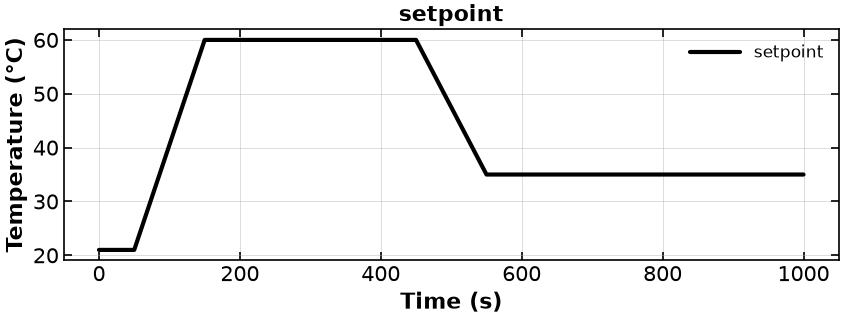
Now let’s solve the optimal control problem to find a control policy for the interval which causes the output to track a desired setpoint or reference trajectory .
# Create a Pyomo model
m = pyo.ConcreteModel("TCLab Heater/Sensor")

# Define time domain
m.t = dae.ContinuousSet(bounds=(0, tf))

# Define the state variables as a function of time
m.Th = pyo.Var(m.t, units=units.kelvin)
m.Ts = pyo.Var(m.t, units=units.kelvin)

# Define the derivatives of the state variables (K/s -- state it explicitly)
m.dTh = dae.DerivativeVar(m.Th, units=units.kelvin / units.s)
m.dTs = dae.DerivativeVar(m.Ts, units=units.kelvin / units.s)

# Define the control variable (heater power) as a function of time
m.u = pyo.Var(m.t, bounds=(0, 100))


# Define the integral of the squared error
@m.Integral(m.t)
def ise(m, t):
    return (units.convert_temp_C_to_K(r(t)) * units.kelvin - m.Th[t]) ** 2


# Define the first differential equation
@m.Constraint(m.t)
def heater1(m, t):
    return (
        CpH * m.dTh[t]
        == Ua * (Tamb - m.Th[t]) + Ub * (m.Ts[t] - m.Th[t]) + alpha * P * m.u[t]
    )


# Define the second differential equation
@m.Constraint(m.t)
def sensor1(m, t):
    return CpS * m.dTs[t] == Ub * (m.Th[t] - m.Ts[t])


# Fix the initial conditions
m.Th[0].fix(Tamb)
m.Ts[0].fix(Tamb)


# Define the objective function
@m.Objective(sense=pyo.minimize)
def objective(m):
    return m.ise


# Units, again checked on the continuous model before discretizing.
assert_units_consistent(m)

# Apply a collocation method to numerically integrate the differential equations
pyo.TransformationFactory("dae.collocation").apply_to(m, nfe=200, wrt=m.t)

# Call our nonlinear optimization/equation solver, Ipopt
results = pyo.SolverFactory("ipopt").solve(m)
assert pyo.check_optimal_termination(results), (
    f"Solve failed: status={results.solver.status}, "
    f"termination={results.solver.termination_condition}"
)

plot_results(m)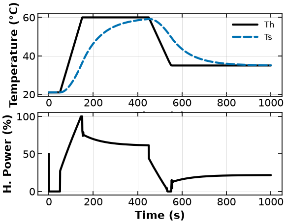
Initialization: start from a physical state
Each TCLab model below fixes the initial heater and sensor temperatures to the measured ambient temperature, Tamb. That is a physical initial condition, not a claim that IPOPT has been given a universally good trajectory guess. For the numerical initialization experiment and a recovery checklist for free-final-time dynamic optimization, see the Race Car example.
Take Away Messages
Pyomo is a great environment to formulate and solve optimization problems.
Predictive models are critical for intelligent decision making.
- Dowling, A. W., Dougher, M., Watson, M. J., Lynch, H. G., Lu, Z., & Laky, D. J. (2025). Teaching Digital Twins in Process Control Using the Temperature Control Lab. Proceedings of the 35th European Symposium on Computer Aided Process Engineering (ESCAPE 35), 4, 2215–2221. 10.69997/sct.180577