Adapted from Pyomo.DAE: Racing Example Revisited and examples
Solver transcripts, mesh evidence, and reproducibility
The two tee=True outputs above are the full IPOPT transcripts for this example. They are useful when you need to inspect the transcribed NLP rather than only the ODE: with Radau collocation (ncp=3) and piecewise-constant controls, the coarse N=10 model has 153 variables and 144 equality constraints; the fine N=100 model has 1503 and 1404. The observed final times are 16.5783 s and 16.4711 s, respectively.
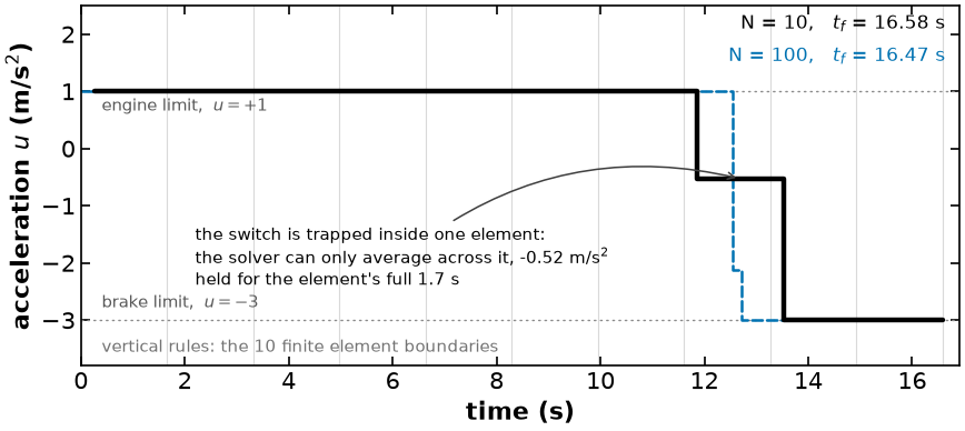
The conclusion is about the mesh, not a universal iteration-count rule: the coarse mesh traps the bang-bang switch inside one element, while the finer mesh resolves it. The stored outputs show one successful run; rerunning the cells is the authoritative way to obtain solver output for your environment. The archived race-car-control and race-car-states result files let the figures be redrawn without rerunning IPOPT.
Learning Objectives
Introduces syntax for Pyomo.DAE
Shows time-scaling modeling trick
Practice using the units feature in Pyomo, and learn where in the workflow to check them (see Units in Pyomo.dae Models)
Install Packages and Load Modules
# Imports
import sys

if "google.colab" in sys.modules:
    !wget "https://raw.githubusercontent.com/ndcbe/optimization/main/notebooks/helper.py"
    import helper

    helper.easy_install()
else:
    sys.path.insert(0, "../")
    import helper
helper.set_plotting_style()
import pyomo.environ as pyo
import matplotlib.pyplot as plt
import pyomo.dae as dae
from pyomo.environ import units
from pyomo.util.check_units import assert_units_consistentProblem Statement and Optimal Control Formulation
You are a race car driver with a simple goal. Drive distance in the minimal amount of time but come to a complete stop at the finish line.
Mathematically, you want to solve the following optimal control problem:
where is the acceleration/braking (your control variable) and is the drag coefficient (parameter).
Declaring our Model with Pyomo.DAE
We can use Pyomo.dae to automatically formulate the collocation equations (i.e., add constraints that numerically integrate the ODE model).
def create_model1():

    # Define the  model
    m = pyo.ConcreteModel()

    # Define the model parameters
    m.R = pyo.Param(initialize=0.001, units=1 / units.m)  # Friction factor
    m.L = pyo.Param(initialize=100.0, units=units.m)  # Final position

    # Define time
    m.tau = dae.ContinuousSet(bounds=(0, 1))  # Dimensionless time set
    m.tf = pyo.Var(initialize=1, units=units.s)  # Final time

    # Define remaining algebraic variables
    m.x = pyo.Var(m.tau, bounds=(0, m.L + 50 * units.m), units=units.m)  # Position
    m.v = pyo.Var(m.tau, bounds=(0, None), units=units.m / units.s)  # Velocity
    m.u = pyo.Var(
        m.tau, bounds=(-3.0, 1.0), initialize=0, units=units.m / units.s / units.s
    )  # Acceleration

    # Define derivative variables.
    #
    # Units MUST be given explicitly: DerivativeVar defaults to dimensionless and
    # does NOT inherit units from the state variable. Because tau is dimensionless,
    # d/dtau has the SAME units as the state itself.
    m.dx = dae.DerivativeVar(m.x, units=units.m)
    m.dv = dae.DerivativeVar(m.v, units=units.m / units.s)

    # Declare the objective (minimize final time)
    m.obj = pyo.Objective(expr=m.tf)

    # Define the constraints
    # position
    @m.Constraint(m.tau)
    def ode1(m, i):
        if i == 0:
            return pyo.Constraint.Skip
        return m.dx[i] == m.tf * m.v[i]

    # velocity
    @m.Constraint(m.tau)
    def ode2(m, i):
        if i == 0:
            return pyo.Constraint.Skip
        return m.dv[i] == m.tf * (m.u[i] - m.R * m.v[i] ** 2)

    # Define the initial/boundary conditions
    def _init(m):
        yield m.x[0] == 0
        yield m.x[1] == m.L
        yield m.v[0] == 0
        yield m.v[1] == 0

    m.initcon = pyo.ConstraintList(rule=_init)

    # Check dimensional consistency HERE, on the continuous model, BEFORE the
    # discretization equations are added. See ./units_and_pyomo_dae.md and
    # https://github.com/Pyomo/pyomo/issues/1790
    assert_units_consistent(m)

    return m


m = create_model1()
Now let’s inspect the model.
m.pprint()2 Param Declarations
L : Size=1, Index=None, Domain=Any, Default=None, Mutable=True, Units=m
Key : Value
None : 100.0
R : Size=1, Index=None, Domain=Any, Default=None, Mutable=True, Units=1/m
Key : Value
None : 0.001
4 Var Declarations
tf : Size=1, Index=None, Units=s
Key : Lower : Value : Upper : Fixed : Stale : Domain
None : None : 1 : None : False : False : Reals
u : Size=2, Index=tau, Units=m/s**2
Key : Lower : Value : Upper : Fixed : Stale : Domain
0 : -3.0 : 0 : 1.0 : False : False : Reals
1 : -3.0 : 0 : 1.0 : False : False : Reals
v : Size=2, Index=tau, Units=m/s
Key : Lower : Value : Upper : Fixed : Stale : Domain
0 : 0 : None : None : False : True : Reals
1 : 0 : None : None : False : True : Reals
x : Size=2, Index=tau, Units=m
Key : Lower : Value : Upper : Fixed : Stale : Domain
0 : 0 : None : 150.0 : False : True : Reals
1 : 0 : None : 150.0 : False : True : Reals
1 Objective Declarations
obj : Size=1, Index=None, Active=True
Key : Active : Sense : Expression
None : True : minimize : tf
3 Constraint Declarations
initcon : Size=4, Index={1, 2, 3, 4}, Active=True
Key : Lower : Body : Upper : Active
1 : 0.0 : x[0] : 0.0 : True
2 : L : x[1] : L : True
3 : 0.0 : v[0] : 0.0 : True
4 : 0.0 : v[1] : 0.0 : True
ode1 : Size=1, Index=tau, Active=True
Key : Lower : Body : Upper : Active
1 : 0.0 : dx[1] - tf*v[1] : 0.0 : True
ode2 : Size=1, Index=tau, Active=True
Key : Lower : Body : Upper : Active
1 : 0.0 : dv[1] - tf*(u[1] - R*v[1]**2) : 0.0 : True
1 ContinuousSet Declarations
tau : Size=1, Index=None, Ordered=Sorted
Key : Dimen : Domain : Size : Members
None : 1 : [0..1] : 2 : {0, 1}
2 DerivativeVar Declarations
dv : Size=2, Index=tau, Units=m/s
Key : Lower : Value : Upper : Fixed : Stale : Domain
0 : None : None : None : False : True : Reals
1 : None : None : None : False : True : Reals
dx : Size=2, Index=tau, Units=m
Key : Lower : Value : Upper : Fixed : Stale : Domain
0 : None : None : None : False : True : Reals
1 : None : None : None : False : True : Reals
13 Declarations: R L tau tf x v u dx dv obj ode1 ode2 initcon
Aside: checking units, and when to check them
Notice where assert_units_consistent(m) sits in create_model1 above: at the very
end of the model-building function, before any discretization is applied.
Two details in the code above are worth pausing on.
DerivativeVardoes not inherit units. It defaults to dimensionless. A model can look thoroughly annotated and still fail the very first check. Before this notebook declaredunits=onm.dxandm.dv,assert_units_consistentfailed immediately withdimensionless not compatible with meter-- even though everyVarandParamhad units.The units of are metres, not metres per second. We scaled time, so is dimensionless and the derivative carries the same units as the state.
That second point has a pleasant consequence, explored in the cell below.
See Units in Pyomo.dae Models for the full story, including what the check does
not look at (Var bounds and .fix() values are never checked).
# The time-scaling trick has a side benefit: because tau is DIMENSIONLESS, the
# finite-difference/collocation coefficients really are dimensionless, so this model
# passes the units check BEFORE and AFTER discretization.
#
# Do not generalize from this! It is a happy accident of scaling time to [0, 1].
# A model whose ContinuousSet is time-in-seconds fails after discretization --
# see notebooks/3/PyomoDAE_TCLab.ipynb for that case.

m_demo = create_model1()  # assert_units_consistent already ran inside
print("Before discretization: units are consistent.")

pyo.TransformationFactory("dae.collocation").apply_to(
    m_demo, nfe=15, scheme="LAGRANGE-RADAU", ncp=3
)

try:
    assert_units_consistent(m_demo)
    print("After discretization:  units are STILL consistent (tau is dimensionless).")
except Exception as e:
    print("After discretization:  FAILED ->", e)
Before discretization: units are consistent.
After discretization: units are STILL consistent (tau is dimensionless).
Discretize/Transcribe and Solve
Pyomo.dae writes the collocation equations for us. The only knob that matters
below is nfe, the number of finite elements: it does not change the model,
only how finely the discretization can resolve it. We solve the same model on
two meshes and compare.
Notice what tee=True prints before the iteration table -- Ipopt reports how
many variables and equality constraints the collocation equations produced.
That count, not the size of the ODE, is what the solver actually sees.
# COARSE mesh: N = 10 finite elements.
#
# N = 10 is chosen, not arbitrary. The optimal control here is bang-bang: full
# throttle (u = +1) until one switching time, then full braking (u = -3) to the
# line. At N = 10 that switching time falls strictly INSIDE a finite element,
# and because reduce_collocation_points holds u constant across an element, the
# only way the discretized problem can say "switch part-way through this
# element" is to give the WHOLE element an intermediate value. Watch for it
# below: one element sits at u = -0.52 m/s^2 for 1.7 s -- a braking level the
# true optimal control never uses. That is an artifact of the mesh, not physics.

NFE_COARSE = 10

m_coarse = create_model1()

# Declare the discretizer
discretizer = pyo.TransformationFactory("dae.collocation")
discretizer.apply_to(m_coarse, nfe=NFE_COARSE, scheme="LAGRANGE-RADAU", ncp=3)

# force piecewise constant controls (acceleration) over each finite element
m_coarse = discretizer.reduce_collocation_points(
    m_coarse, var=m_coarse.u, ncp=1, contset=m_coarse.tau
)

# Solve. tee=True prints Ipopt's own log: first the problem-size block -- how
# many variables and equality constraints the collocation equations produced --
# and then the iteration table.
solver = pyo.SolverFactory("ipopt")
solve_status = solver.solve(m_coarse, tee=True)
assert pyo.check_optimal_termination(solve_status), (
    f"Solve failed: status={solve_status.solver.status}, "
    f"termination={solve_status.solver.termination_condition}"
)

print("final time = %6.2f seconds" % (pyo.value(m_coarse.tf)))
Ipopt 3.13.2:
******************************************************************************
This program contains Ipopt, a library for large-scale nonlinear optimization.
Ipopt is released as open source code under the Eclipse Public License (EPL).
For more information visit http://projects.coin-or.org/Ipopt
This version of Ipopt was compiled from source code available at
https://github.com/IDAES/Ipopt as part of the Institute for the Design of
Advanced Energy Systems Process Systems Engineering Framework (IDAES PSE
Framework) Copyright (c) 2018-2019. See https://github.com/IDAES/idaes-pse.
This version of Ipopt was compiled using HSL, a collection of Fortran codes
for large-scale scientific computation. All technical papers, sales and
publicity material resulting from use of the HSL codes within IPOPT must
contain the following acknowledgement:
HSL, a collection of Fortran codes for large-scale scientific
computation. See http://www.hsl.rl.ac.uk.
******************************************************************************
This is Ipopt version 3.13.2, running with linear solver ma27.
Number of nonzeros in equality constraint Jacobian...: 554
Number of nonzeros in inequality constraint Jacobian.: 0
Number of nonzeros in Lagrangian Hessian.............: 90
Total number of variables............................: 153
variables with only lower bounds: 31
variables with lower and upper bounds: 61
variables with only upper bounds: 0
Total number of equality constraints.................: 144
Total number of inequality constraints...............: 0
inequality constraints with only lower bounds: 0
inequality constraints with lower and upper bounds: 0
inequality constraints with only upper bounds: 0
iter objective inf_pr inf_du lg(mu) ||d|| lg(rg) alpha_du alpha_pr ls
0 1.0000000e+00 1.00e+02 1.21e+00 -1.0 0.00e+00 - 0.00e+00 0.00e+00 0
1r 1.0000000e+00 1.00e+02 9.99e+02 2.0 0.00e+00 - 0.00e+00 4.95e-07R 7
2r 1.2919636e+00 9.95e+01 9.92e+02 2.0 1.38e+02 - 6.81e-03 7.19e-03f 1
3r 2.5914422e+00 9.91e+01 2.32e+02 0.6 1.70e+00 - 6.02e-01 7.66e-01f 1
4r 2.9428748e+00 9.89e+01 2.00e+02 0.6 5.01e-01 2.0 6.24e-01 8.58e-01f 1
5r 5.0335018e+00 9.80e+01 1.76e+02 -0.1 4.45e+01 - 5.29e-02 5.86e-02f 1
6r 5.0495684e+00 9.78e+01 8.55e+01 -0.1 1.06e+00 1.5 1.89e-01 6.09e-01f 1
7r 8.6702058e+00 9.58e+01 2.96e+02 -0.1 5.32e+02 - 4.65e-04 6.80e-03f 1
8r 9.9255513e+00 9.43e+01 6.94e+01 -0.1 2.21e+00 1.0 7.78e-01 1.00e+00f 1
9r 3.2512069e+01 7.28e+01 7.37e+02 -0.1 2.68e+01 - 2.37e-01 1.00e+00f 1
iter objective inf_pr inf_du lg(mu) ||d|| lg(rg) alpha_du alpha_pr ls
10 3.5220013e+01 5.48e+01 2.18e+00 -1.0 2.63e+02 - 1.66e-01 2.48e-01h 3
11 3.5764409e+01 5.32e+01 1.01e+01 -1.0 3.72e+02 - 3.77e-01 2.98e-02h 5
12 3.5851359e+01 5.28e+01 3.17e+01 -1.0 3.32e+02 - 6.09e-01 6.02e-03h 8
13 3.5896997e+01 5.26e+01 6.07e+01 -1.0 2.85e+02 - 8.16e-01 3.87e-03h 9
14 3.5904346e+01 5.26e+01 9.65e+01 -1.0 2.28e+02 - 1.00e+00 9.67e-04h 11
15 1.4582615e+01 6.12e+01 7.30e+00 -1.0 1.14e+02 -4.0 3.14e-01 7.59e-01f 1
16 1.9843491e+01 2.14e+01 1.29e+01 -1.0 9.06e+01 - 6.05e-01 7.07e-01h 1
17 1.7728032e+01 1.46e+01 2.88e+02 -1.0 4.61e+01 - 9.35e-01 3.51e-01h 1
18 1.9088612e+01 9.06e+00 1.95e+02 -1.0 1.57e+02 - 4.22e-01 3.94e-01h 1
19 1.9144571e+01 1.63e-01 2.95e+02 -1.0 5.05e+01 - 7.60e-01 9.90e-01f 1
iter objective inf_pr inf_du lg(mu) ||d|| lg(rg) alpha_du alpha_pr ls
20 1.8483294e+01 7.50e-02 1.09e+03 -1.0 3.06e+01 - 1.00e+00 9.91e-01H 1
21 1.8532962e+01 1.02e-02 8.99e-05 -1.0 3.33e+00 - 1.00e+00 1.00e+00h 1
22 1.7025414e+01 2.23e+00 1.30e+06 -3.8 1.48e+01 - 7.85e-01 1.00e+00f 1
23 1.6686749e+01 3.85e-01 9.84e+04 -3.8 3.97e+00 - 9.25e-01 8.96e-01h 1
24 1.6583461e+01 2.54e-02 1.23e-04 -3.8 3.21e+00 - 1.00e+00 1.00e+00h 1
25 1.6582355e+01 2.32e-06 1.06e-08 -3.8 1.74e-02 - 1.00e+00 1.00e+00h 1
26 1.6578350e+01 2.24e-05 4.43e-07 -5.7 4.83e-02 - 1.00e+00 1.00e+00h 1
27 1.6578347e+01 1.86e-11 1.85e-11 -5.7 6.56e-05 - 1.00e+00 1.00e+00h 1
28 1.6578297e+01 3.46e-09 6.83e-11 -8.6 6.00e-04 - 1.00e+00 1.00e+00f 1
Number of Iterations....: 28
(scaled) (unscaled)
Objective...............: 1.6578296960737259e+01 1.6578296960737259e+01
Dual infeasibility......: 6.8311969554225784e-11 6.8311969554225784e-11
Constraint violation....: 3.4584957120387116e-09 3.4584957120387116e-09
Complementarity.........: 2.5548433389337429e-09 2.5548433389337429e-09
Overall NLP error.......: 3.4584957120387116e-09 3.4584957120387116e-09
Number of objective function evaluations = 77
Number of objective gradient evaluations = 22
Number of equality constraint evaluations = 77
Number of inequality constraint evaluations = 0
Number of equality constraint Jacobian evaluations = 30
Number of inequality constraint Jacobian evaluations = 0
Number of Lagrangian Hessian evaluations = 28
Total CPU secs in IPOPT (w/o function evaluations) = 0.008
Total CPU secs in NLP function evaluations = 0.000
EXIT: Optimal Solution Found.
final time = 16.58 seconds
Finer Time Discretization
Does the intermediate braking force go away if we consider a finer time discretization?
# FINE mesh: N = 100 finite elements.
#
# The same problem on a mesh ten times finer. Nothing about the model changes;
# only nfe does. The switching element is still there -- it always is, because
# the switch almost never lands exactly on an element boundary -- but it is now
# 0.16 s wide instead of 1.7 s, so the control profile looks like the bang-bang
# solution it is approximating, and the objective stops moving.

NFE_FINE = 100

m_fine = create_model1()

# Declare the discretizer
discretizer = pyo.TransformationFactory("dae.collocation")
discretizer.apply_to(m_fine, nfe=NFE_FINE, scheme="LAGRANGE-RADAU", ncp=3)

# force piecewise constant controls (acceleration) over each finite element
m_fine = discretizer.reduce_collocation_points(
    m_fine, var=m_fine.u, ncp=1, contset=m_fine.tau
)

# Solve. tee=True prints Ipopt's own log: first the problem-size block -- how
# many variables and equality constraints the collocation equations produced --
# and then the iteration table.
solver = pyo.SolverFactory("ipopt")
solve_status = solver.solve(m_fine, tee=True)
assert pyo.check_optimal_termination(solve_status), (
    f"Solve failed: status={solve_status.solver.status}, "
    f"termination={solve_status.solver.termination_condition}"
)

print("final time = %6.2f seconds" % (pyo.value(m_fine.tf)))
Ipopt 3.13.2:
******************************************************************************
This program contains Ipopt, a library for large-scale nonlinear optimization.
Ipopt is released as open source code under the Eclipse Public License (EPL).
For more information visit http://projects.coin-or.org/Ipopt
This version of Ipopt was compiled from source code available at
https://github.com/IDAES/Ipopt as part of the Institute for the Design of
Advanced Energy Systems Process Systems Engineering Framework (IDAES PSE
Framework) Copyright (c) 2018-2019. See https://github.com/IDAES/idaes-pse.
This version of Ipopt was compiled using HSL, a collection of Fortran codes
for large-scale scientific computation. All technical papers, sales and
publicity material resulting from use of the HSL codes within IPOPT must
contain the following acknowledgement:
HSL, a collection of Fortran codes for large-scale scientific
computation. See http://www.hsl.rl.ac.uk.
******************************************************************************
This is Ipopt version 3.13.2, running with linear solver ma27.
Number of nonzeros in equality constraint Jacobian...: 5504
Number of nonzeros in inequality constraint Jacobian.: 0
Number of nonzeros in Lagrangian Hessian.............: 900
Total number of variables............................: 1503
variables with only lower bounds: 301
variables with lower and upper bounds: 601
variables with only upper bounds: 0
Total number of equality constraints.................: 1404
Total number of inequality constraints...............: 0
inequality constraints with only lower bounds: 0
inequality constraints with lower and upper bounds: 0
inequality constraints with only upper bounds: 0
iter objective inf_pr inf_du lg(mu) ||d|| lg(rg) alpha_du alpha_pr ls
0 1.0000000e+00 1.00e+02 2.27e+00 -1.0 0.00e+00 - 0.00e+00 0.00e+00 0
1 3.0401570e+00 1.00e+02 1.60e+00 -1.0 1.16e+04 - 9.91e-05 1.75e-04f 2
2 4.9319942e-01 9.92e+01 1.57e+03 -1.0 6.53e+02 0.0 1.56e-04 8.05e-03f 1
3 8.9105198e-01 9.90e+01 1.51e+03 -1.0 8.18e+02 - 3.04e-03 1.54e-03f 1
4 1.7090653e+00 9.85e+01 8.01e+02 -1.0 4.75e+02 - 6.66e-03 5.25e-03h 1
5 3.2434604e+00 9.67e+01 5.11e+02 -1.0 2.50e+02 - 1.53e-02 1.85e-02f 1
6 5.0004772e+00 9.29e+01 4.91e+02 -1.0 1.88e+02 - 2.29e-02 3.89e-02f 1
7 1.5105802e+01 6.15e+01 1.95e+03 -1.0 1.82e+02 -0.5 4.32e-02 3.38e-01f 1
8 1.5307639e+01 6.02e+01 1.91e+03 -1.0 1.36e+02 -1.0 1.78e-02 2.08e-02f 1
9 1.5360072e+01 5.98e+01 1.89e+03 -1.0 9.42e+01 -0.5 9.02e-03 6.69e-03h 1
iter objective inf_pr inf_du lg(mu) ||d|| lg(rg) alpha_du alpha_pr ls
10 1.5664835e+01 5.96e+01 1.89e+03 -1.0 1.14e+03 -1.0 3.32e-04 2.62e-03f 1
11 1.5924852e+01 5.83e+01 1.84e+03 -1.0 9.80e+01 -0.6 9.06e-03 2.27e-02f 1
12 1.5937832e+01 5.82e+01 1.84e+03 -1.0 8.22e+01 -0.2 1.49e-02 1.56e-03h 1
13 1.7583117e+01 5.27e+01 1.62e+03 -1.0 9.88e+01 -0.6 4.77e-03 9.44e-02f 1
14 1.7604366e+01 5.26e+01 1.62e+03 -1.0 7.24e+01 -0.2 2.99e-02 2.19e-03h 1
15 2.0811793e+01 4.37e+01 1.24e+03 -1.0 8.80e+01 -0.7 1.15e-02 1.69e-01f 1
16 2.3547909e+01 4.26e+01 1.20e+03 -1.0 4.22e+02 -1.2 8.14e-03 2.45e-02h 1
17 2.4207206e+01 4.04e+01 1.13e+03 -1.0 6.43e+01 -0.7 1.50e-01 5.29e-02h 1
18 3.2543819e+01 2.76e+01 6.05e+02 -1.0 1.19e+02 -1.2 3.47e-01 3.15e-01h 1
19 3.4480258e+01 2.27e+01 4.92e+02 -1.0 7.25e+01 -1.7 9.91e-01 1.81e-01h 1
iter objective inf_pr inf_du lg(mu) ||d|| lg(rg) alpha_du alpha_pr ls
20 3.9509586e+01 1.62e+00 6.71e+01 -1.0 3.53e+01 -1.3 5.80e-01 9.90e-01h 1
21 3.9921946e+01 1.05e-01 4.35e+02 -1.0 8.94e+00 -1.7 8.92e-01 9.90e-01h 1
  22  3.6362628e+01 1.46e+00 9.35e+04  -1.0 5.53e+02    -  2.53e-01 4.03e-02f  1
  23  3.6118968e+01 1.76e-02 3.88e-02  -1.0 2.17e+00  -2.2 1.00e+00 1.00e+00f  1
  24  1.8378466e+01 4.38e+01 1.79e+03  -3.8 2.69e+03    -  4.01e-02 3.69e-02f  1
  25  1.5215375e+01 3.35e+01 2.33e+05  -3.8 7.92e+01    -  4.80e-03 4.44e-01h  1
  26  1.7890203e+01 2.54e+00 4.80e+05  -3.8 2.13e+01    -  6.56e-02 9.49e-01h  1
  27  1.7667756e+01 9.11e-02 3.88e+04  -3.8 6.04e+00    -  9.22e-01 1.00e+00h  1
  28  1.6829488e+01 1.39e+00 1.55e+04  -3.8 2.94e+01    -  5.99e-01 9.44e-01h  1
  29  1.6614032e+01 3.34e-01 4.95e+03  -3.8 2.29e+01    -  6.81e-01 8.75e-01h  1
iter    objective    inf_pr   inf_du lg(mu)  ||d||  lg(rg) alpha_du alpha_pr  ls
  30  1.6538014e+01 1.20e-01 1.51e+03  -3.8 2.66e+01    -  6.95e-01 8.59e-01h  1
  31  1.6517013e+01 1.80e-02 1.99e+02  -3.8 1.42e+01    -  8.68e-01 1.00e+00h  1
  32  1.6515413e+01 6.12e-04 3.73e-08  -3.8 6.32e+00    -  1.00e+00 1.00e+00h  1
  33  1.6472038e+01 1.23e-02 1.22e+03  -5.7 4.66e+00    -  9.18e-01 1.00e+00h  1
  34  1.6471688e+01 5.61e-06 2.69e-09  -5.7 2.67e-01    -  1.00e+00 1.00e+00h  1
  35  1.6471138e+01 1.74e-06 7.86e-09  -8.6 5.09e-02    -  1.00e+00 1.00e+00h  1
  36  1.6471138e+01 1.21e-11 2.55e-14  -8.6 1.51e-04    -  1.00e+00 1.00e+00h  1

Number of Iterations....: 36

                                   (scaled)                 (unscaled)
Objective...............:   1.6471137966472515e+01    1.6471137966472515e+01
Dual infeasibility......:   2.5492694953627627e-14    2.5492694953627627e-14
Constraint violation....:   2.0090432312482888e-12    1.2109227372780665e-11
Complementarity.........:   2.5059164913864815e-09    2.5059164913864815e-09
Overall NLP error.......:   2.5059164913864815e-09    2.5059164913864815e-09


Number of objective function evaluations             = 39
Number of objective gradient evaluations             = 37
Number of equality constraint evaluations            = 39
Number of inequality constraint evaluations          = 0
Number of equality constraint Jacobian evaluations   = 37
Number of inequality constraint Jacobian evaluations = 0
Number of Lagrangian Hessian evaluations             = 36
Total CPU secs in IPOPT (w/o function evaluations)   =      0.098
Total CPU secs in NLP function evaluations           =      0.005

EXIT: Optimal Solution Found.
final time = 16.47 seconds
Comparing the Two Meshes
Both solves are done, so pull the trajectories out of the two models and
archive them. Separating “solve” from “analyze” is a habit worth keeping: the
plotting cells below then depend only on results, and can be re-run without a
solver.
def extract_race_car_results(m, nfe):
    """Pull the solved trajectories out of a Pyomo model into plain lists.

    Arguments:
        m: solved, discretized race-car model
        nfe: number of finite elements used, for the label

    Returns:
        dict of JSON-safe values -- everything the figures need and nothing else

    The time axis is rebuilt here: the model is written in dimensionless time
    tau in [0, 1], so physical time is t = tau * t_f, and t_f is itself a
    decision variable. Two meshes therefore have DIFFERENT final times, which
    is the number the mesh-refinement argument turns on.
    """
    tf = pyo.value(m.tf)
    tau = sorted(m.tau)
    return {
        "label": f"N = {nfe}",
        "nfe": nfe,
        "tf": tf,
        "t": [i * tf for i in tau],  # time [s]
        "x": [pyo.value(m.x[i]) for i in tau],  # position [m]
        "v": [pyo.value(m.v[i]) for i in tau],  # velocity [m/s]
        "u": [pyo.value(m.u[i]) for i in tau],  # acceleration [m/s^2]
        # Element boundaries in physical time, so a figure can show WHERE the
        # control is allowed to change value.
        "elements": [b * tf for b in m.tau.get_finite_elements()],
    }


results = {
    "meshes": [
        extract_race_car_results(m_coarse, NFE_COARSE),
        extract_race_car_results(m_fine, NFE_FINE),
    ],
    "u_lower": -3.0,  # [m/s^2]
    "u_upper": 1.0,  # [m/s^2]
    "L": 100.0,  # [m]
}

for mesh in results["meshes"]:
    print(f"{mesh['label']:>8}:  t_f = {mesh['tf']:.4f} s")

DESCRIPTION = (
    "Minimum-time race car (m = 1, L = 100 m, drag R = 0.001 1/m, "
    "-3 <= u <= 1), solved with Pyomo.dae LAGRANGE-RADAU collocation, ncp = 3, "
    "with the control reduced to piecewise constant on each element. Two "
    "meshes: N = 10, coarse enough that the bang-bang switch is trapped inside "
    "one element and that element takes an intermediate braking value, and "
    "N = 100, where the switch is resolved."
)

for figure_name in ("race-car-control", "race-car-states"):
    helper.save_results(
        figure_name,
        results,
        notebook="notebooks/3-dev/PyomoDAE_car.ipynb",
        source_tag="handout:race-car-model",
        description=DESCRIPTION,
        solver="Ipopt 3.13.2 (IDAES build, linear solver ma27)",
    )
N = 10: t_f = 16.5783 s
N = 100: t_f = 16.4711 s
[helper] wrote figures/results/race-car-control.json
[helper] wrote figures/results/race-car-states.json
The control profile
This is where the two meshes disagree.
# This cell is tagged `figure:race-car-control', which makes it the single
# source of the control-profile figure the Lecture 7 handout prints.
# figures/render_from_notebook.py re-runs exactly this cell against the archived
# JSON when the house style changes, so there is no second copy of the plotting
# code. That driver binds `np', `plt' and `helper' for the cell, so it imports
# nothing and uses no name defined in an earlier cell except `results'.


def plot_race_car_control(results):
    """The control profile on both meshes, and what the coarse mesh gets wrong.

    THE FIGURE'S POINT is the flat step at u ~ -0.5 in the coarse profile. The
    exact solution is bang-bang -- it takes only the two bound values -- so any
    element sitting between them is the discretization confessing that it put
    the switching time inside an element and had to average across it. On the
    fine mesh the same element is a tenth as wide and the profile reads as the
    step function it approximates.

    STEPS, NOT LINES. The control really is piecewise constant over an element
    (that is what reduce_collocation_points enforces), so drawstyle="steps-post"
    draws what the NLP contains. A plain line would interpolate diagonally
    across the switch and show a smooth ramp that no variable in the model
    represents.

    ⚠ tau = 0 IS DROPPED from the control series. u[0] is not a control the
    solver uses -- the reduced control is indexed by element, and the first
    element's value lives at its first collocation point -- so plotting u[0]
    puts a spurious step from its initialize=0 value at the left edge.

    ELEMENT RULES, coarse mesh only. The light vertical lines are the finite
    element boundaries: the control is constant between two of them by
    construction, so the rules explain the staircase rather than decorating it.
    Drawing them for N = 100 would be a grey block.

    GREYSCALE. Two series, each taking colour AND linestyle together from the
    house prop_cycle (figures/dowling.mplstyle pairs the two element-wise),
    plus different line widths, plus a direct label beside each curve. Any one
    of those is enough on a photocopy.
    """
    meshes = results["meshes"]
    coarse = meshes[0]
    u_lo, u_hi = results["u_lower"], results["u_upper"]
    t_max = max(m["tf"] for m in meshes)
    colors = plt.rcParams["axes.prop_cycle"].by_key()["color"]

    fig, ax = plt.subplots(figsize=(9.0, 4.2))

    # Element boundaries FIRST, so they sit under the data.
    for b in coarse["elements"]:
        ax.axvline(b, color="0.85", linewidth=0.8, zorder=0)

    for u_bound in (u_hi, u_lo):
        ax.axhline(
            u_bound, color="0.55", linewidth=1.0, linestyle=(0, (1, 3)), zorder=1
        )

    for k, mesh in enumerate(meshes):
        t = mesh["t"][1:]
        u = mesh["u"][1:]
        ax.plot(
            t, u, drawstyle="steps-post", linewidth=3.2 if k == 0 else 1.8, zorder=3 - k
        )

    # The defect, called out where it happens. Exactly one coarse element sits
    # strictly between the bounds; find it rather than hard-coding a time.
    tol = 1e-3
    trapped = [
        (t, u)
        for t, u in zip(coarse["t"][1:], coarse["u"][1:])
        if u_lo + tol < u < u_hi - tol
    ]
    if trapped:
        t_bad = trapped[len(trapped) // 2][0]
        u_bad = trapped[0][1]
        ax.annotate(
            "the switch is trapped inside one element:\n"
            f"the solver can only average across it, {u_bad:+.2f} m/s$^2$\n"
            f"held for the element's full {coarse['tf'] / coarse['nfe']:.1f} s",
            xy=(t_bad, u_bad),
            xytext=(0.13, 0.30),
            textcoords="axes fraction",
            ha="left",
            va="center",
            fontsize=11,
            arrowprops=dict(
                arrowstyle="->",
                linewidth=1.1,
                color="0.25",
                connectionstyle="arc3,rad=-0.25",
            ),
        )

    # DIRECT LABELS, not a legend: the two profiles coincide for most of the
    # horizon, so a legend box would sit somewhere the eye has to travel to.
    # They go ABOVE the engine-limit line -- headroom made by the ylim below,
    # because every other corner of these axes has a curve or a rule in it.
    for k, mesh in enumerate(meshes):
        ax.annotate(
            f"{mesh['label']},   $t_f$ = {mesh['tf']:.2f} s",
            xy=(0.985, 0.95 - 0.09 * k),
            xycoords="axes fraction",
            ha="right",
            va="center",
            fontsize=12.5,
            color=colors[k],
        )

    ax.annotate(
        "engine limit,  $u = +1$",
        xy=(0.4, u_hi - 0.12),
        ha="left",
        va="top",
        fontsize=10.5,
        color="0.35",
    )
    ax.annotate(
        "brake limit,  $u = -3$",
        xy=(0.4, u_lo + 0.14),
        ha="left",
        va="bottom",
        fontsize=10.5,
        color="0.35",
    )
    ax.annotate(
        f"vertical rules: the {coarse['nfe']} finite element boundaries",
        xy=(0.4, u_lo - 0.62),
        ha="left",
        va="bottom",
        fontsize=10.5,
        color="0.45",
    )

    ax.set_xlabel("time (s)")
    ax.set_ylabel(r"acceleration $u$ (m/s$^2$)")
    ax.set_xlim(0, t_max * 1.02)
    ax.set_ylim(u_lo - 0.8, u_hi + 1.5)
    fig.tight_layout()
    return fig


fig = plot_race_car_control(results)

# Write media/figures/race-car-control.{png,pdf} -- what the lecture handout
# \includegraphics. A no-op on Colab, where there is no repo to write to.
helper.save_figure(fig, "race-car-control")
[helper] wrote media/figures/race-car-control.png and .pdf
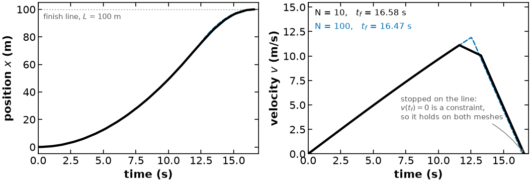
The state trajectories
And this is where they agree -- which is the trap.
# Tagged `figure:race-car-states': the single source of the state-trajectory
# figure in the Lecture 7 handout. Same contract as the cell above -- it uses
# only `results', `plt' and `helper', and defines its own figsize.


def plot_race_car_states(results):
    """Position and velocity on both meshes.

    WHY THIS FIGURE SITS BESIDE THE CONTROL FIGURE. That one shows where the
    coarse discretization goes wrong; this one shows how little of it reaches
    the states. Position is visually identical on the two meshes, and the coarse
    solution still lands exactly on x = L with v = 0 -- because those are
    constraints, and a constraint holds on any mesh. What the coarse mesh gets
    wrong is the OBJECTIVE. A student reading only these two panels would
    conclude N = 10 was fine.

    THE VELOCITY PANEL IS WHERE THE DEFECT IS VISIBLE. The trapped element's
    weak braking rounds the peak of the coarse velocity curve where the fine one
    turns sharply, and the coarse car then brakes at the limit for longer to
    still stop on the line.

    GREYSCALE. Colour and linestyle move together from the house prop_cycle,
    the line widths differ, and the labels are direct rather than a legend.
    """
    meshes = results["meshes"]
    colors = plt.rcParams["axes.prop_cycle"].by_key()["color"]
    t_max = max(m["tf"] for m in meshes)

    fig, (ax_x, ax_v) = plt.subplots(1, 2, figsize=(11.0, 4.0))

    ax_x.axhline(
        results["L"], color="0.55", linewidth=1.0, linestyle=(0, (1, 3)), zorder=1
    )
    for k, mesh in enumerate(meshes):
        style = dict(linewidth=3.2 if k == 0 else 1.8, zorder=3 - k)
        ax_x.plot(mesh["t"], mesh["x"], **style)
        ax_v.plot(mesh["t"], mesh["v"], **style)

    ax_x.annotate(
        f"finish line, $L$ = {results['L']:.0f} m",
        xy=(0.4, results["L"] - 3),
        ha="left",
        va="top",
        fontsize=10.5,
        color="0.35",
    )

    # Both labels go in the empty upper-left wedge of the velocity panel, above
    # the acceleration ramp and left of the peak.
    for k, mesh in enumerate(meshes):
        ax_v.annotate(
            f"{mesh['label']},   $t_f$ = {mesh['tf']:.2f} s",
            xy=(0.03, 0.93 - 0.09 * k),
            xycoords="axes fraction",
            ha="left",
            va="center",
            fontsize=12.5,
            color=colors[k],
        )

    ax_v.annotate(
        "stopped on the line:\n$v(t_f) = 0$ is a constraint,\nso it holds on both meshes",
        xy=(meshes[0]["tf"], 0.0),
        xytext=(0.42, 0.30),
        textcoords="axes fraction",
        ha="left",
        va="center",
        fontsize=10.5,
        color="0.35",
        arrowprops=dict(
            arrowstyle="->",
            linewidth=1.0,
            color="0.45",
            connectionstyle="arc3,rad=-0.2",
        ),
    )

    ax_x.set_xlabel("time (s)")
    ax_x.set_ylabel("position $x$ (m)")
    ax_v.set_xlabel("time (s)")
    ax_v.set_ylabel("velocity $v$ (m/s)")
    for ax in (ax_x, ax_v):
        ax.set_xlim(0, t_max * 1.02)
    ax_v.set_ylim(0, max(max(m["v"]) for m in meshes) * 1.30)
    fig.tight_layout()
    return fig


fig = plot_race_car_states(results)
helper.save_figure(fig, "race-car-states")
[helper] wrote media/figures/race-car-states.png and .pdf
Discussion Questions
Do the results make sense? What do you know about the relationships between position, velocity, and acceleration? Do you see those relationships in the plots?
The coarse mesh satisfies every constraint exactly and still reports a final time 0.6% too large. Which quantity would you monitor to decide that a mesh is fine enough -- the constraint violations, or the objective?
Initialization experiment
Good initial values are useful insurance, but this small, well-scaled race-car model is a useful counterexample to the claim that a poor guess must fail. The following five runs use create_model1, N=15, ncp=3, LAGRANGE-RADAU, and no reduce_collocation_points call. All converged to the same final time.
| Initial values | IPOPT iterations | (s) |
|---|---|---|
| default () | 81 | 16.4708 |
| all states 0; | 81 | 16.4708 |
| all states 0; ; | 79 | 16.4708 |
| all states 0; ; no lower bound | 98 | 16.4708 |
| all states 0; | 44 | 16.4708 |
These results were recorded with IPOPT 3.13.2 and ma27. They show that the solver can move this model away from a degenerate guess; they do not show that initialization is unimportant. A different Pyomo/IPOPT or linear-solver version, operating system, processor, scaling, or model/mesh can change iteration counts and even the behavior near a zero lower bound. To reproduce or extend the experiment, keep the configuration above fixed, record the environment, and alter one initial-value choice at a time.
For a more difficult dynamic optimization problem, start with physical state values, bound scalars such as final time away from a degenerate value, simulate before optimizing when possible, and solve a coarse mesh before refining it.
Another Version
Another modeling option is to define an extra differential equation to compute time. The normalized-time formulation is unchanged: tau remains the fixed independent variable on , and tf remains a decision variable. The additional state is useful when physical time must be available along the trajectory; otherwise, recover it after solving as .
def create_model2():

    # Define the  model
    m = pyo.ConcreteModel()

    # Define the model parameters
    m.R = pyo.Param(initialize=0.001, units=1 / units.m)  # Friction factor
    m.L = pyo.Param(initialize=100.0, units=units.m)  # Final position

    # Define time
    m.tau = dae.ContinuousSet(bounds=(0, 1))  # Dimensionless time set
    m.time = pyo.Var(m.tau, bounds=(0, None), units=units.s)  # Time
    m.tf = pyo.Var(initialize=1, units=units.s)  # Final time

    # Define remaining algebraic variables
    m.x = pyo.Var(m.tau, bounds=(0, m.L + 50 * units.m), units=units.m)  # Position
    m.v = pyo.Var(m.tau, bounds=(0, None), units=units.m / units.s)  # Velocity
    m.u = pyo.Var(
        m.tau, bounds=(-3.0, 1.0), initialize=0, units=units.m / units.s / units.s
    )  # Acceleration

    # Define derivative variables. tau is dimensionless, so d/dtau carries the
    # same units as the state. DerivativeVar does not infer these -- say them.
    m.dtime = dae.DerivativeVar(m.time, units=units.s)
    m.dx = dae.DerivativeVar(m.x, units=units.m)
    m.dv = dae.DerivativeVar(m.v, units=units.m / units.s)

    # Declare the objective (minimize final time)
    m.obj = pyo.Objective(expr=m.tf)

    # Define the constraints
    # position
    @m.Constraint(m.tau)
    def ode1(m, i):
        if i == 0:
            return pyo.Constraint.Skip
        return m.dx[i] == m.tf * m.v[i]

    # velocity
    @m.Constraint(m.tau)
    def ode2(m, i):
        if i == 0:
            return pyo.Constraint.Skip
        return m.dv[i] == m.tf * (m.u[i] - m.R * m.v[i] ** 2)

    # time
    @m.Constraint(m.tau)
    def ode3(m, i):
        if i == 0:
            return pyo.Constraint.Skip
        return m.dtime[i] == m.tf

    # Define the initial/boundary conditions
    def _init(m):
        yield m.x[0] == 0
        yield m.x[1] == m.L
        yield m.v[0] == 0
        yield m.v[1] == 0
        yield m.time[0] == 0

    m.initcon = pyo.ConstraintList(rule=_init)

    # Units are checked on the continuous model, before discretization.
    assert_units_consistent(m)

    return m


m = create_model2()
# Declare the discretizer
discretizer = pyo.TransformationFactory("dae.collocation")
discretizer.apply_to(m, nfe=15, scheme="LAGRANGE-RADAU", ncp=3)
# force piecewise constant controls (acceleration) over each finite element
m = discretizer.reduce_collocation_points(m, var=m.u, ncp=1, contset=m.tau)
# Solve
solver = pyo.SolverFactory("ipopt")
results = solver.solve(m, tee=True)
assert pyo.check_optimal_termination(results), (
f"Solve failed: status={results.solver.status}, "
f"termination={results.solver.termination_condition}"
)
print("final time = %6.2f seconds" % (pyo.value(m.tf)))Ipopt 3.13.2:
******************************************************************************
This program contains Ipopt, a library for large-scale nonlinear optimization.
Ipopt is released as open source code under the Eclipse Public License (EPL).
For more information visit http://projects.coin-or.org/Ipopt
This version of Ipopt was compiled from source code available at
https://github.com/IDAES/Ipopt as part of the Institute for the Design of
Advanced Energy Systems Process Systems Engineering Framework (IDAES PSE
Framework) Copyright (c) 2018-2019. See https://github.com/IDAES/idaes-pse.
This version of Ipopt was compiled using HSL, a collection of Fortran codes
for large-scale scientific computation. All technical papers, sales and
publicity material resulting from use of the HSL codes within IPOPT must
contain the following acknowledgement:
HSL, a collection of Fortran codes for large-scale scientific
computation. See http://www.hsl.rl.ac.uk.
******************************************************************************
This is Ipopt version 3.13.2, running with linear solver ma27.
Number of nonzeros in equality constraint Jacobian...: 1145
Number of nonzeros in inequality constraint Jacobian.: 0
Number of nonzeros in Lagrangian Hessian.............: 135
Total number of variables............................: 319
variables with only lower bounds: 92
variables with lower and upper bounds: 91
variables with only upper bounds: 0
Total number of equality constraints.................: 305
Total number of inequality constraints...............: 0
inequality constraints with only lower bounds: 0
inequality constraints with lower and upper bounds: 0
inequality constraints with only upper bounds: 0
iter objective inf_pr inf_du lg(mu) ||d|| lg(rg) alpha_du alpha_pr ls
0 1.0000000e+00 1.00e+02 3.48e-01 -1.0 0.00e+00 - 0.00e+00 0.00e+00 0
1 9.9965381e-01 9.99e+01 1.09e+02 -1.0 1.00e+03 - 7.69e-05 1.26e-03f 1
2 1.0672606e+00 9.98e+01 1.21e+02 -1.0 8.13e+02 - 1.78e-04 1.13e-03f 1
3 1.6627950e+00 9.94e+01 3.76e+01 -1.0 6.32e+02 - 4.66e-04 3.48e-03f 1
4 2.1580706e+00 9.89e+01 2.13e+01 -1.0 3.70e+02 - 5.94e-03 4.73e-03f 1
5 3.3740442e+00 9.75e+01 2.13e+01 -1.0 2.83e+02 - 6.48e-03 1.47e-02f 1
6 3.4568065e+00 9.75e+01 2.12e+01 -1.0 3.65e+03 -2.0 9.05e-05 2.25e-04f 4
7 3.5166768e+00 9.75e+01 2.12e+01 -1.0 1.45e+05 -1.6 3.05e-07 2.70e-06f 4
8 3.6179009e+00 9.74e+01 2.11e+01 -1.0 4.56e+02 -1.1 6.90e-03 7.57e-04h 4
9 3.7394769e+00 9.74e+01 2.10e+01 -1.0 2.14e+03 -1.6 4.01e-04 2.70e-04h 3
iter objective inf_pr inf_du lg(mu) ||d|| lg(rg) alpha_du alpha_pr ls
10 3.9133700e+00 9.72e+01 2.10e+01 -1.0 3.70e+02 -1.2 1.66e-02 1.41e-03h 3
11 4.4185485e+00 9.71e+01 1.98e+01 -1.0 1.58e+03 - 2.59e-03 1.55e-03h 1
12 4.5952693e+00 9.69e+01 1.98e+01 -1.0 4.16e+02 - 5.05e-03 1.57e-03h 1
13 4.9840028e+00 9.66e+01 1.97e+01 -1.0 4.67e+02 - 7.60e-03 3.38e-03h 1
14 5.3631837e+00 9.61e+01 1.98e+01 -1.0 2.80e+02 - 6.53e-03 5.27e-03h 1
15 5.8588385e+00 9.55e+01 1.96e+01 -1.0 3.63e+02 - 7.97e-03 5.72e-03h 2
16 6.2740527e+00 9.51e+01 1.96e+01 -1.0 4.21e+02 - 1.56e-02 4.53e-03h 1
17 6.6359047e+00 9.45e+01 2.20e+01 -1.0 2.85e+02 - 1.32e-02 6.28e-03h 1
18 7.1860006e+00 9.36e+01 2.75e+01 -1.0 3.17e+02 - 1.47e-02 9.08e-03h 4
19 7.8876904e+00 9.27e+01 2.76e+01 -1.0 4.06e+02 - 1.29e-02 9.78e-03h 2
iter objective inf_pr inf_du lg(mu) ||d|| lg(rg) alpha_du alpha_pr ls
20 8.3302999e+00 9.20e+01 2.73e+01 -1.0 3.73e+02 - 7.91e-03 7.33e-03h 2
21 8.7005071e+00 9.15e+01 3.38e+01 -1.0 3.73e+02 - 1.67e-03 5.55e-03h 1
22 8.8614541e+00 9.12e+01 3.54e+01 -1.0 3.10e+02 - 1.44e-02 3.62e-03h 1
23 9.3754873e+00 9.01e+01 3.94e+01 -1.0 3.09e+02 - 1.59e-02 1.18e-02h 1
24 1.0173832e+01 8.84e+01 3.85e+01 -1.0 3.05e+02 - 4.92e-02 1.97e-02h 3
25 1.1806583e+01 8.59e+01 5.17e+01 -1.0 3.68e+02 -1.7 4.14e-03 2.80e-02h 2
26 1.3077594e+01 8.20e+01 3.75e+01 -1.0 2.75e+02 -1.3 6.22e-02 4.47e-02h 3
27 1.3909957e+01 8.03e+01 2.75e+01 -1.0 3.28e+02 -1.7 6.11e-02 2.12e-02h 3
28 1.4861686e+01 7.65e+01 3.46e+01 -1.0 2.40e+02 -1.3 2.30e-02 4.78e-02f 3
29 1.5847144e+01 7.35e+01 3.03e+01 -1.0 2.70e+02 -1.8 9.50e-02 3.85e-02h 5
iter objective inf_pr inf_du lg(mu) ||d|| lg(rg) alpha_du alpha_pr ls
30 1.7199412e+01 7.22e+01 2.99e+01 -1.0 5.15e+02 -2.3 2.07e-02 1.84e-02h 1
31 1.7264467e+01 7.20e+01 4.19e+01 -1.0 2.86e+02 - 1.06e-01 2.56e-03h 1
32 3.3947489e+01 5.88e+00 1.98e+02 -1.0 2.70e+02 - 7.07e-02 9.22e-01H 1
33 3.3892282e+01 7.53e-02 7.75e+01 -1.0 1.50e+01 -1.8 5.55e-01 9.90e-01h 1
34 3.1099781e+01 3.25e+00 4.34e+02 -1.0 2.09e+02 - 1.62e-01 1.83e-01f 1
35 3.3257932e+01 1.99e+00 9.45e+03 -1.0 2.87e+01 - 5.56e-01 9.92e-01f 1
36 3.0676688e+01 3.10e+00 1.40e+06 -1.0 3.75e+01 - 2.66e-01 9.12e-01f 1
37 2.8971974e+01 1.94e+00 5.27e+06 -1.0 3.39e+01 - 2.61e-01 1.00e+00f 1
38 2.7979354e+01 1.41e+00 9.55e+05 -1.0 2.59e+01 - 7.48e-01 5.84e-01h 1
39 2.5272864e+01 5.18e+00 1.26e+06 -1.0 1.17e+02 - 1.27e-01 5.83e-01f 1
iter objective inf_pr inf_du lg(mu) ||d|| lg(rg) alpha_du alpha_pr ls
40 2.5693827e+01 3.44e-01 1.27e+06 -1.0 2.11e+01 - 2.36e-01 1.00e+00f 1
41 2.2982818e+01 4.74e+00 7.78e+05 -1.0 9.26e+01 - 3.86e-01 6.26e-01f 1
42 2.0165927e+01 6.73e+00 5.59e+05 -1.0 6.11e+01 - 2.81e-01 8.52e-01f 1
43 1.8548643e+01 5.04e+00 3.42e+05 -1.0 6.52e+01 - 3.89e-01 5.46e-01f 1
44 1.9691536e+01 1.01e+00 4.17e-02 -1.0 1.57e+01 - 1.00e+00 1.00e+00f 1
45 1.9758985e+01 5.69e-02 3.33e-03 -1.0 1.62e+01 - 1.00e+00 1.00e+00h 1
46 1.7116764e+01 5.67e+00 2.62e+06 -2.5 2.17e+01 - 7.30e-01 1.00e+00f 1
47 1.6751093e+01 3.80e-01 9.60e+04 -2.5 1.33e+01 - 9.63e-01 1.00e+00h 1
48 1.6637572e+01 4.98e-02 8.50e-05 -2.5 7.31e+00 - 1.00e+00 1.00e+00h 1
49 1.6637598e+01 7.09e-07 2.95e-08 -2.5 1.37e-01 - 1.00e+00 1.00e+00h 1
iter objective inf_pr inf_du lg(mu) ||d|| lg(rg) alpha_du alpha_pr ls
50 1.6521647e+01 2.19e-02 1.17e+04 -5.7 1.83e+00 - 9.59e-01 1.00e+00f 1
51 1.6520272e+01 3.39e-06 4.17e-08 -5.7 2.75e-02 - 1.00e+00 1.00e+00h 1
52 1.6520192e+01 9.39e-09 1.64e-10 -8.6 1.01e-03 - 1.00e+00 1.00e+00h 1
Number of Iterations....: 52
(scaled) (unscaled)
Objective...............: 1.6520191520761482e+01 1.6520191520761482e+01
Dual infeasibility......: 1.6444812999846882e-10 1.6444812999846882e-10
Constraint violation....: 9.3907885911903577e-09 9.3907885911903577e-09
Complementarity.........: 2.5872224352029850e-09 2.5872224352029850e-09
Overall NLP error.......: 9.3907885911903577e-09 9.3907885911903577e-09
Number of objective function evaluations = 110
Number of objective gradient evaluations = 53
Number of equality constraint evaluations = 110
Number of inequality constraint evaluations = 0
Number of equality constraint Jacobian evaluations = 53
Number of inequality constraint Jacobian evaluations = 0
Number of Lagrangian Hessian evaluations = 52
Total CPU secs in IPOPT (w/o function evaluations) = 0.026
Total CPU secs in NLP function evaluations = 0.002
EXIT: Optimal Solution Found.
final time = 16.52 seconds