Prepared by: Prof. Alexander Dowling (2026)
This notebook is the PDE companion to Lecture 7. We take one transient conduction problem,
write it for three geometries at once, discretize space with the method of lines, and solve
the resulting differential-algebraic system with Pyomo.dae.
The physical problem and the idea of indexing the three geometries with a single shape parameter are adapted from J. C. Kantor, ND Pyomo Cookbook, notebook 5.03 “Heat Conduction in Various Geometries”. The derivation, the code and the numerical experiments below are our own.
# Install Pyomo and solvers for Google Colab
import sys

if "google.colab" in sys.modules:
    !wget "https://raw.githubusercontent.com/ndcbe/optimization/main/notebooks/helper.py"
    import helper

    helper.easy_install()
else:
    sys.path.insert(0, "../")
    import helper
helper.set_plotting_style()

import numpy as np
import matplotlib.pyplot as plt
import pyomo.environ as pyo
import pyomo.dae as dae
from pyomo.util.model_size import build_model_size_report
from scipy.special import j0, j1, jn_zeros
Learning Objectives
Nondimensionalize a transient conduction PDE and recognize the Fourier number as its only time scale
Write one model that covers a slab, a cylinder and a sphere through a shape index
Apply the method of lines: discretize space first, then hand a DAE in time to
Pyomo.daeCompare finite difference, finite volume and finite element spatial discretizations, and say where each belongs
Handle the coordinate singularity correctly
Run the IDAES Diagnostics Toolbox on a
Pyomo.daemodel and read its report -- including the difference between a warning and a cautionRecognize a dangling variable: a derivative that appears in no discretization equation, which IPOPT will happily declare
optimal
The Physical Problem
A solid body, initially at uniform temperature , is dropped at into a bath held at . The surface reaches the bath temperature immediately, and we want the temperature everywhere inside as a function of time.
With constant thermal conductivity , density and heat capacity , and no source term, the energy balance is
Divide by and define the thermal diffusivity , which has units of length/time:
One Equation, Three Geometries
The three classical bodies -- an infinite slab of half-thickness , an infinite cylinder of radius , and a sphere of radius -- are all one-dimensional: temperature depends on a single space coordinate measured from the center. In each case the Laplacian of a radially symmetric field is
where the shape index is
| Geometry | measured from | Surface at | |
|---|---|---|---|
| Slab (infinite plate, half-thickness ) | 0 | the midplane | |
| Cylinder (infinite, radius ) | 1 | the axis | |
| Sphere (radius ) | 2 | the center |
For the slab, and the extra term vanishes -- Cartesian coordinates. For and the geometry contributes the term, which is singular at the center. That singularity is the interesting part of this notebook, so hold onto it.
Nondimensionalization
Three scales are available: the temperature difference the body must cross, the body’s own size, and the time the heat needs to cross it. Define
Substituting, with , and :
Every term carries the same factor , which therefore cancels:
with
Two things are worth noticing.
No parameters survive. The dimensionless problem depends only on . Solve it once per geometry and you have solved it for every material, every size and every pair of temperatures.
is the Fourier number, : the ratio of the time elapsed to the time heat needs to diffuse across the body. is “thoroughly heated.”
The last condition is the symmetry (or no-flux) condition. It is not an extra physical assumption -- it follows from the body being symmetric about , so no heat can cross the center. It is, however, the boundary condition that will cause all the trouble.
From here on we drop the primes and write , , for the dimensionless quantities.
The Method of Lines
We have one equation in two independent variables. Pyomo.dae is comfortable with either, but
the standard strategy for a parabolic PDE is to break the symmetry between them:
Method of lines. Discretize the spatial derivatives on a fixed mesh . What is left is a system of ODEs (here, a DAE, because the boundary rows are algebraic) in time alone, one equation per mesh point -- the “lines” of the name.
Writing , the semi-discrete system is
with the discrete approximation to at node , plus algebraic rows at (symmetry) and (the bath temperature).
Why this order?
The time direction is an initial-value problem, and Lecture 7’s machinery -- orthogonal collocation on finite elements -- is built exactly for that. We can hand the time direction to
dae.collocationand get a high-order, stiffly stable integrator for free.The space direction is a boundary-value problem in disguise. All of its structure -- the boundary conditions, the coordinate singularity, the conservation properties -- is decided by how we build . Doing it deliberately, rather than letting a transformation do it for us, is the whole game.
In Pyomo.dae both directions are ContinuousSets and both get a TransformationFactory, so the
method of lines is a way of thinking about the model rather than a different API. But it tells you
which transformation to worry about.
Three Ways to Discretize Space
All three families replace by a sparse linear operator on nodal values. They differ in what they ask the approximation to reproduce exactly, and that choice is what makes one appropriate and another awkward for a given problem.
Finite difference (FD): match the Taylor series
Pick a stencil and choose coefficients so the truncation error is as high order as possible. On a uniform mesh of spacing ,
Cheap and transparent. Every row is three numbers. This is what
dae.finite_differencebuilds.Appropriate when the geometry is simple, the mesh is structured, and the coefficients (, ) are smooth.
Awkward when you need a guarantee. FD approximates the differential equation pointwise; it makes no promise that the discrete system conserves energy, and it has nothing to say at a point where the differential equation itself is singular -- such as here.
Finite volume (FV): match the integral balance
Partition the domain into control volumes (here, shells) and integrate the conservation law over each one. Using the self-adjoint form and integrating over the cell ,
Approximating each face gradient by a two-point difference gives a scheme in which the flux leaving one cell is identically the flux entering the next, so the sum over cells telescopes: the scheme conserves energy to machine precision on any mesh, coarse or fine.
Appropriate when conservation matters (reactors, flow, shocks), the mesh is unstructured, or the coefficients jump at an interface -- FV puts the interface on a face, where the flux is single valued.
Note what it does at : the inner face of the first cell has area for . The symmetry condition is structural: no special case, no boundary condition to write. We will use this below.
Finite element (FE): match a weighted residual
Expand in basis functions and require the residual to be orthogonal to a set of test functions. Galerkin FE integrates the weak form by parts, which lowers the smoothness the solution must have and produces symmetric, provably stable operators; orthogonal collocation, the variant used throughout Lecture 7, instead forces the residual to vanish exactly at a set of collocation points inside each element.
Appropriate when the geometry is complicated, the solution is smooth enough to reward high order, or you want error estimates and adaptivity on a rigorous footing.
In
Pyomo.daethis isdae.collocation. We use it in time below. It can also be applied in space -- and, as we will see, it inherits exactly the same trap as the finite difference scheme.
The Coordinate Singularity at 
For the term is undefined at . The solution is perfectly well behaved there -- by symmetry at least as fast as , so L’Hopital’s rule gives -- but the equation as written cannot be evaluated at . Two consequences for the discrete model:
Never write the PDE row at . In Pyomo, return
pyo.Constraint.Skip. The row that takes its place is the symmetry condition , which is what makes the center temperature well posed.Skip the corner . The initial condition asks for there and the boundary condition asks for . Both cannot hold. We keep the boundary condition (the bath is imposed from onward) and skip the initial condition at . Physically this is the discontinuity that makes the surface flux infinite at ; numerically it is simply one row we must not write twice.
The second point is routine bookkeeping. The first one hides a trap.
A Pyomo.dae Model
Here is the model, written once for all three geometries. Read the three constraint rules first -- they are a direct transcription of the boxed PDE and its three side conditions.
A Pyomo.dae Model
Here is the model, written once for all three geometries. Read the three constraint rules first -- they are a direct transcription of the boxed PDE and its three side conditions. Then read the block after the transformations, which supplies the one equation the spatial discretization does not write for us. The next section explains why it is needed and what happens without it.
def build_fd(s, nfe_r, tf=0.5, nfe_t=30, ncp=3):
    """Transient conduction in a slab (s=0), cylinder (s=1) or sphere (s=2).

    Space: finite difference, CENTRAL, nfe_r elements on r in [0, 1], plus a
           second-order one-sided row at r = 0 for the symmetry condition.
    Time:  orthogonal collocation on finite elements (Radau), nfe_t elements, ncp points.

    Arguments:
        s: shape index. 0 = slab, 1 = cylinder, 2 = sphere.
        nfe_r: number of spatial finite elements.
        tf: final dimensionless time (Fourier number).
        nfe_t, ncp: time discretization.

    Returns:
        A ConcreteModel, already discretized, ready to solve. Zero degrees of freedom.
    """
    m = pyo.ConcreteModel()

    # Two continuous sets: dimensionless time and dimensionless radius
    m.t = dae.ContinuousSet(bounds=(0, tf))
    m.r = dae.ContinuousSet(bounds=(0, 1))

    # Dimensionless temperature and its derivatives.
    # Everything here is dimensionless by construction, so there are no Pyomo
    # units to carry -- see [](./units_and_pyomo_dae.md) for the case where there are.
    m.T = pyo.Var(m.t, m.r, initialize=0.0)
    m.dTdt = dae.DerivativeVar(m.T, wrt=m.t)
    m.dTdr = dae.DerivativeVar(m.T, wrt=m.r)
    m.d2Tdr2 = dae.DerivativeVar(m.T, wrt=(m.r, m.r))

    @m.Constraint(m.t, m.r)
    def pde(m, t, r):
        # Skip t=0: the initial condition owns that row.
        # Skip r=0: the s/r term is singular there. The symmetry condition takes its place.
        # Skip r=1: the bath temperature owns that row.
        if t == 0 or r == 0 or r == 1:
            return pyo.Constraint.Skip
        return m.dTdt[t, r] == m.d2Tdr2[t, r] + (s / r) * m.dTdr[t, r]

    @m.Constraint(m.r)
    def ic(m, r):
        # Skip the corner (t, r) = (0, 1): the boundary condition wins there.
        if r == 1:
            return pyo.Constraint.Skip
        return m.T[0, r] == 0

    @m.Constraint(m.t)
    def bc_surface(m, t):
        return m.T[t, 1] == 1

    # --- discretize -------------------------------------------------------
    pyo.TransformationFactory("dae.finite_difference").apply_to(
        m, wrt=m.r, nfe=nfe_r, scheme="CENTRAL"
    )
    pyo.TransformationFactory("dae.collocation").apply_to(
        m, wrt=m.t, nfe=nfe_t, ncp=ncp, scheme="LAGRANGE-RADAU"
    )

    # --- symmetry at the center, AFTER discretization ---------------------
    # The mesh only exists once the transformation has run, and the stencil below
    # names specific mesh points.
    #
    # The symmetry condition is TWO statements, and CENTRAL gives us neither:
    #   (1) dTdr[t, 0] is zero                       -- the physics, imposed by fixing
    #   (2) dTdr[t, 0] is tied to the temperatures   -- the equation CENTRAL never wrote
    # Omitting (2) leaves dTdr[t, 0] dangling and the center temperature unconstrained.
    rs = sorted(m.r)
    h = rs[1] - rs[0]

    for t in m.t:
        m.dTdr[t, 0].fix(0)  # (1) symmetry; fixing removes a variable instead of adding a row

    @m.Constraint(m.t)
    def bc_center_def(m, t):
        # (2) second-order three-point one-sided stencil:
        #     dT/dr|_0 = (-3 T_0 + 4 T_1 - T_2) / (2h) + O(h^2)
        if t == 0:
            return pyo.Constraint.Skip  # the initial condition already pins this row
        return m.dTdr[t, 0] * (2 * h) == (
            -3 * m.T[t, rs[0]] + 4 * m.T[t, rs[1]] - m.T[t, rs[2]]
        )

    # A simulation, not an optimization: a constant objective keeps IPOPT happy.
    m.obj = pyo.Objective(expr=0.0)
    return m


def solve_model(m, tee=False):
    """Solve with IPOPT and report the termination condition without asserting on it.

    We deliberately do NOT assert optimality here: half the point of this notebook is
    that `optimal` is not the same as `correct`.
    """
    results = pyo.SolverFactory("ipopt").solve(m, tee=tee)
    return results.solver.termination_condition
The Trap: A Derivative That Appears in No Equation
Everything in build_fd up to the transformations is a transcription of the mathematics. The block
after them is not, and it is the part that is easy to leave out. Here is the natural way to write the
symmetry condition:
@m.Constraint(m.t)
def bc_center(m, t):
    return m.dTdr[t, 0] == 0        # DO NOT DO THIS AND NOTHING ELSE
It reads exactly like . It is also wrong, for a reason that has nothing
to do with the mathematics and everything to do with what scheme="CENTRAL" actually generates.
A central difference needs a neighbour on both sides. At an interior node it has one:
At there is no , so Pyomo.dae writes no equation at all for .
It is not set to a one-sided difference; it is not set to anything. It is a variable that appears in
no discretization equation -- a dangling variable. The constraint above would then not impose
symmetry on the temperature field; it would assign a value to a number that touches nothing else in
the model, and the center temperature would be determined by nothing at all.
We can see the hole directly, without building a model at all. Discretize a bare DerivativeVar and
ask which mesh points the generated defining equations cover.
def stencil_coverage(scheme, nfe=4):
    """Which mesh points does dae.finite_difference give a defining equation to?

    A probe of the transformation, not a model of anything: one variable, its first
    and second derivatives, no PDE and no boundary conditions.
    """
    p = pyo.ConcreteModel()
    p.r = dae.ContinuousSet(bounds=(0, 1))
    p.T = pyo.Var(p.r)
    p.dTdr = dae.DerivativeVar(p.T, wrt=p.r)
    p.d2Tdr2 = dae.DerivativeVar(p.T, wrt=(p.r, p.r))
    pyo.TransformationFactory("dae.finite_difference").apply_to(p, wrt=p.r, nfe=nfe, scheme=scheme)
    mesh = set(p.r)
    return (sorted(mesh - set(p.dTdr_disc_eq.keys())),
            sorted(mesh - set(p.d2Tdr2_disc_eq.keys())))


print("mesh points on r in [0, 1] with nfe=4:", [f"{v:g}" for v in np.linspace(0, 1, 5)], "\n")
print(f"{'scheme':10s} {'r with NO dT/dr equation':>28s} {'r with NO d2T/dr2 equation':>30s}")
for scheme in ["CENTRAL", "FORWARD", "BACKWARD"]:
    miss1, miss2 = stencil_coverage(scheme)
    print(f"{scheme:10s} {str(miss1):>28s} {str(miss2):>30s}")
mesh points on r in [0, 1] with nfe=4: ['0', '0.25', '0.5', '0.75', '1']
scheme r with NO dT/dr equation r with NO d2T/dr2 equation
CENTRAL [0, 1] [0, 1]
FORWARD [1] [0.75, 1]
BACKWARD [0] [0, 0.25]
Read the CENTRAL row: neither endpoint gets a defining equation for the first derivative, and neither
gets one for the second. At that is harmless -- the PDE row is skipped there and the bath
temperature is imposed directly. At it is fatal, because the PDE row is skipped there too.
The other two rows are the reason “just use a one-sided scheme everywhere” is not a fix: FORWARD and
BACKWARD each close one hole and open another somewhere else. They move the problem rather than solve
it. See the first table below.
So build_fd writes both halves of the symmetry condition itself: it fixes to
zero, which is the physics, and it adds bc_center_def, which is the equation the scheme never wrote.
Together with the three-point stencil collapses to , the
second-order statement that the profile is flat at the center.
The Reference Solution
Each of the three geometries has a classical separation-of-variables solution, so we can measure error rather than eyeball it. For the dimensionless problem above:
def analytic(s, t, r, nterms=400):
    """Series solution of the dimensionless problem. Returns an array over r."""
    r = np.atleast_1d(np.asarray(r, dtype=float))
    out = np.zeros_like(r)
    if s == 0:
        n = np.arange(1, nterms)
        lam = (2 * n - 1) * np.pi / 2
        for k, rr in enumerate(r):
            out[k] = 1 - np.sum(2 * (-1) ** (n + 1) / lam * np.cos(lam * rr) * np.exp(-(lam**2) * t))
    elif s == 1:
        b = jn_zeros(0, nterms)
        for k, rr in enumerate(r):
            out[k] = 1 - np.sum(2 * j0(b * rr) * np.exp(-(b**2) * t) / (b * j1(b)))
    elif s == 2:
        n = np.arange(1, nterms)
        for k, rr in enumerate(r):
            if rr < 1e-12:  # the r -> 0 limit of sin(n pi r)/r
                out[k] = 1 + np.sum(2 * (-1) ** n * np.exp(-((n * np.pi) ** 2) * t))
            else:
                out[k] = 1 + (2 / (np.pi * rr)) * np.sum(
                    ((-1) ** n / n) * np.sin(n * np.pi * rr) * np.exp(-((n * np.pi) ** 2) * t)
                )
    else:
        raise ValueError("s must be 0, 1 or 2")
    return out


GEOMETRY = {0: "Slab", 1: "Cylinder", 2: "Sphere"}
Checking the Model Before You Trust It
This is a simulation: the temperature field is completely determined by the data, so a correctly posed model must have zero degrees of freedom. That is the cheapest check available, and it happens before the solver is ever called.
print(f"{'geometry':10s} {'variables':>10s} {'constraints':>12s} {'DOF':>6s}")
for s in [0, 1, 2]:
    report = build_model_size_report(build_fd(s=s, nfe_r=40)).activated
    dof = report["variables"] - report["constraints"]
    print(f"{GEOMETRY[s]:10s} {report['variables']:10d} {report['constraints']:12d} {dof:6d}")
geometry variables constraints DOF
Slab 14519 14519 0
Cylinder 14519 14519 0
Sphere 14519 14519 0
The IDAES Diagnostics Toolbox
Counting degrees of freedom tells you how many variables are unaccounted for. It does not tell you which. On a model with tens of thousands of rows that difference is the whole game, so run the structural analysis rather than the arithmetic.
The IDAES Diagnostics Toolbox
does exactly this. report_structural_issues() needs no solution and no initialization -- it works on
the incidence pattern of the model, so you can run it the moment the model is built. Make it the first
thing you do to any Pyomo.dae model, before you ever look at a number.
from idaes.core.util.diagnostics_tools.diagnostics_toolbox import DiagnosticsToolbox

# A small model so the report is readable; the structural conclusions do not depend on mesh size.
DiagnosticsToolbox(build_fd(s=0, nfe_r=8, nfe_t=4)).report_structural_issues()
====================================================================================
Model Statistics
Activated Blocks: 1 (Deactivated: 0)
Free Variables in Activated Constraints: 407 (External: 0)
Free Variables with only lower bounds: 0
Free Variables with only upper bounds: 0
Free Variables with upper and lower bounds: 0
Fixed Variables in Activated Constraints: 12 (External: 0)
Activated Equality Constraints: 407 (Deactivated: 0)
Activated Inequality Constraints: 0 (Deactivated: 0)
Activated Objectives: 1 (Deactivated: 0)
------------------------------------------------------------------------------------
0 WARNINGS
No warnings found!
------------------------------------------------------------------------------------
2 Cautions
Caution: 13 variables fixed to 0
Caution: 49 unused variables (1 fixed)
------------------------------------------------------------------------------------
Suggested next steps:
Try to initialize/solve your model and then call report_numerical_issues()
====================================================================================
Zero warnings. No structural singularity, no under-constrained set, no over-constrained set,
degrees of freedom consistent with the constraint count. That is what a well-posed Pyomo.dae model
looks like.
The two cautions are worth understanding, because they are not defects and you will see them on every model of this shape.
13 variables fixed to 0-- these are at the 13 time points, fixed bybuild_fdas statement (1) of the symmetry condition. The toolbox flags variables fixed to zero because a strayfix(0)is a common way to accidentally delete physics. Here it is the physics.49 unused variables-- variables that appear in no activated constraint. All 49 are inert: 9 are at , which Radau collocation never references; 26 are on the two boundary rows and , where the PDE is skipped; and 14 are at the surface and at , likewise unreferenced.Pyomo.daecreates a full grid of derivative variables and only some of them are used. They influence no result.
A caution is an invitation to look, not a finding. Knowing which cautions your model should produce is what lets you notice the day it produces a different one.
Alternative Discretizations at , and What They Do
The table below documents the discretizations we did not ship, so that the failure modes are on record without a broken model being a copy-paste away.
All numbers were measured on the slab () unless stated, at , with
nfe_t=30, ncp=3 Radau collocation in time, and IPOPT 3.13.2 with ma27. “Center error” is
with ; the five values run over
and “order” is of the ratio of the last two.
| Alternative discretization at | Modeling issue | Failure evidence (measured) |
|---|---|---|
scheme="CENTRAL" with dTdr[t,0] == 0 as the only center row (no defining equation) | Dangling variable. CENTRAL emits no defining equation for a derivative at an endpoint, so dTdr[t,0] appears in no discretization row. The constraint assigns a value to a variable that touches nothing; the center temperature is constrained by nothing. | DOF = 90 at nfe_r=40 -- one spare degree of freedom per time point at which the PDE is enforced. report_structural_issues() reports “Structural singularity found” with an under-constrained set of 360 variables and 348 constraints (at nfe_r=8, nfe_t=4). Center error plateaus: 0.739, 0.731, 0.726, 0.724, 0.722, observed order 0.00 -- refinement does nothing, because there is no equation to converge. The answer is arbitrary: initial guesses of 0.0, 0.5 and -2.0 give , -0.0703 and -0.2667 against an exact 0.6292. All three solves returned optimal, and all three are negative absolute temperatures on a 0--1 scale. 🔴 Silent on the cylinder and the sphere -- see the note below. |
scheme="FORWARD" for the whole interior, as a way to get a definition at | Moves the hole. FORWARD does define both derivatives at , but its second-derivative stencil runs off the right end of the domain instead: the last interior node loses its defining equation, and that node carries a real PDE row. | The coverage probe above: CENTRAL leaves undefined at and ; FORWARD at the last interior node and ; BACKWARD at and the first interior node. No single one-sided scheme covers every node that needs one. |
First-order one-sided center row, dTdr[t,0]*h == T[t,r1] - T[t,r0] (with dTdr[t,0] fixed, i.e. ) | Correct but low order. No dangling variable, DOF = 0, converges. But the center row is while the interior is , and the boundary row caps the accuracy of the whole scheme. | Center error 0.047, 0.023, 0.0115, 0.0057, 0.0029 -- observed order 1.00. The shipped three-point row on the same meshes: 6.6e-5, 3.1e-5, 9.4e-6, 2.6e-6, 6.7e-7 -- observed order 1.94, four orders of magnitude better on the finest mesh. |
✅ Shipped: scheme="CENTRAL" interior + fixed dTdr[t,0] + second-order three-point center row | The scheme’s missing equation is supplied explicitly, at the same order as the interior. | DOF = 0, 0 warnings from report_structural_issues(), observed order 1.94, and initialization-independent (next cell). Solves at scale: nfe_r=160, nfe_t=30 is 58,604 variables, DOF 0, optimal in 4.0 s, . |
The Answer Does Not Depend on the Initial Guess
A model with unconstrained degrees of freedom and no objective has no unique answer, and the quickest way to see that is to change the initial guess and re-solve. Run the same check on the correct model: if the answer moves, something is not pinned.
print(f"{'geometry':10s} {'nfe_r':>6s}" + "".join(f"{'guess ' + str(g):>14s}" for g in [0.0, 0.5, -2.0])
      + f"{'exact':>12s}")
for s in [0, 1, 2]:
    exact = analytic(s, 0.5, 0.0)[0]
    for n in [10, 20, 40]:
        row = []
        for guess in [0.0, 0.5, -2.0]:
            m = build_fd(s=s, nfe_r=n)
            for v in m.T.values():
                v.set_value(guess)
            solve_model(m)
            row.append(pyo.value(m.T[0.5, 0]))
        print(f"{GEOMETRY[s]:10s} {n:6d}" + "".join(f"{v:14.6f}" for v in row) + f"{exact:12.6f}")
geometry nfe_r guess 0.0 guess 0.5 guess -2.0 exact
Slab 10 0.629157 0.629157 0.629157 0.629223
Slab 20 0.629192 0.629192 0.629192 0.629223
Slab 40 0.629213 0.629213 0.629213 0.629223
Cylinder 10 0.910245 0.910245 0.910245 0.911110
Cylinder 20 0.910885 0.910885 0.910885 0.911110
Cylinder 40 0.911053 0.911053 0.911053 0.911110
Sphere 10 0.985151 0.985151 0.985151 0.985616
Sphere 20 0.985500 0.985500 0.985500 0.985616
Sphere 40 0.985587 0.985587 0.985587 0.985616
Identical to every digit printed across a range of guesses that includes a physically impossible one, in every
geometry and on every mesh. The remaining discrepancy against exact is truncation error, and unlike
a structural defect it goes away under refinement -- which is what the next section measures.
Mesh Refinement Tells the Truth
A structural defect does not announce itself in a single solve. It announces itself under refinement: a consistent scheme’s error must go to zero with , and an underdetermined one’s does not have to. This is the check that turns “the model ran” into evidence.
NFE_LIST = [10, 20, 40, 80, 160]
TF = 0.5

conv = {}
convergence_rows = []
for s in [0, 1, 2]:
    exact = analytic(s, TF, 0.0)[0]
    errs = []
    for n in NFE_LIST:
        m = build_fd(s=s, nfe_r=n)
        solve_model(m)
        errs.append(abs(pyo.value(m.T[TF, 0]) - exact))
    conv[s] = np.array(errs)
    convergence_rows.append({
        "shape_index": s,
        "geometry": GEOMETRY[s],
        "exact_center_temperature": exact,
        "errors": errs,
        "observed_order": float(np.log2(errs[-2] / errs[-1])),
    })

initial_guess_rows = []
for s in [0, 1, 2]:
    exact = analytic(s, TF, 0.0)[0]
    for n in [10, 20, 40]:
        values = []
        for guess in [0.0, 0.5, -2.0]:
            m = build_fd(s=s, nfe_r=n)
            for v in m.T.values():
                v.set_value(guess)
            solve_model(m)
            values.append(pyo.value(m.T[TF, 0]))
        initial_guess_rows.append({
            "shape_index": s,
            "geometry": GEOMETRY[s],
            "nfe_r": n,
            "initial_guesses": [0.0, 0.5, -2.0],
            "center_temperatures": values,
            "exact_center_temperature": exact,
        })

convergence_results = {
    "nfe_r": NFE_LIST,
    "final_fourier_number": TF,
    "geometries": convergence_rows,
    "initial_guess_experiment": initial_guess_rows,
    "diagnostics": {
        "model": "build_fd(s=0, nfe_r=8, nfe_t=4)",
        "warnings": 0,
        "expected_cautions": [
            "13 variables fixed to 0",
            "49 unused variables (1 fixed)",
        ],
    },
}
helper.save_results(
    "heat-convergence",
    convergence_results,
    notebook="notebooks/3-dev/heat_conduction_pde.ipynb",
    description=(
        "Center-temperature spatial-refinement errors for the shipped finite-"
        "difference heat-conduction model in slab, cylinder and sphere geometries; "
        "also records the initial-guess experiment and the expected structural "
        "diagnostics for the model."
    ),
    solver="Ipopt 3.13.2 (IDAES build, linear solver ma27); Pyomo 6.10.1",
)
results = convergence_results

print(f"|T(t_f, 0) - exact|   at   t_f = {TF}")
print(f"  {'':9s}" + "".join(f"{'h=1/'+str(n):>12s}" for n in NFE_LIST) + f"{'order':>9s}")
for row in convergence_rows:
    print(f"  {row['geometry']:9s}" + "".join(f"{v:12.3e}" for v in row["errors"])
          + f"{row['observed_order']:9.2f}")
[helper] wrote figures/results/heat-convergence.json
|T(t_f, 0) - exact|   at   t_f = 0.5
                 h=1/10      h=1/20      h=1/40      h=1/80     h=1/160    order
  Slab        6.573e-05   3.075e-05   9.391e-06   2.557e-06   6.653e-07     1.94
  Cylinder    8.651e-04   2.256e-04   5.707e-05   1.432e-05   3.582e-06     2.00
  Sphere      4.656e-04   1.164e-04   2.910e-05   7.275e-06   1.819e-06     2.00
Read the order column: it is of the ratio of the last two errors, so 2.0 means second order
in , 1.0 means first order, and would mean the error is not going anywhere. All three
geometries land at 1.9--2.0, which is what the interior stencil and the center row were each built to
deliver -- and it is only true because they deliver it at the same order. The first-order center row
in the table above produces the same picture with slope 1, and the dangling model produces a flat line.
h = 1.0 / np.asarray(results["nfe_r"], dtype=float)

fig, ax = plt.subplots(figsize=(6.4, 4.8))

MARKERS = {0: "o", 1: "s", 2: "^"}
for row in results["geometries"]:
    s = row["shape_index"]
    errors = np.asarray(row["errors"], dtype=float)
    (line,) = ax.loglog(h, errors, marker=MARKERS[s], markersize=7, lw=2.0)
    # direct labelling: a legend keyed only by colour dies in black and white
    ax.annotate(row["geometry"], xy=(h[-1], errors[-1]), xytext=(8, -4),
                textcoords="offset points", fontsize=11,
                color=line.get_color(), fontweight="bold")

# reference slope, drawn in grey so it never competes with the data
slab_errors = np.asarray(results["geometries"][0]["errors"], dtype=float)
ax.loglog(h, slab_errors[0] * (h / h[0]) ** 2, color="0.6", lw=1.5,
          ls=(0, (2, 2)), zorder=0)
ax.annotate("slope 2", xy=(h[2], slab_errors[0] * (h[2] / h[0]) ** 2),
            xytext=(-52, -6), textcoords="offset points", fontsize=11, color="0.4")

ax.set_xlabel("mesh spacing $h$")
ax.set_ylabel("center error")
ax.set_xlim(h[-1] / 2.2, h[0] * 1.5)
ax.set_title("Center-temperature error under spatial mesh refinement")

# Write media/figures/heat-convergence.{png,pdf} -- what the lecture handout
# \includegraphics. A no-op on Colab, where there is no repo to write to.
helper.save_figure(fig, "heat-convergence")
plt.show()
[helper] wrote media/figures/heat-convergence.png and .pdf
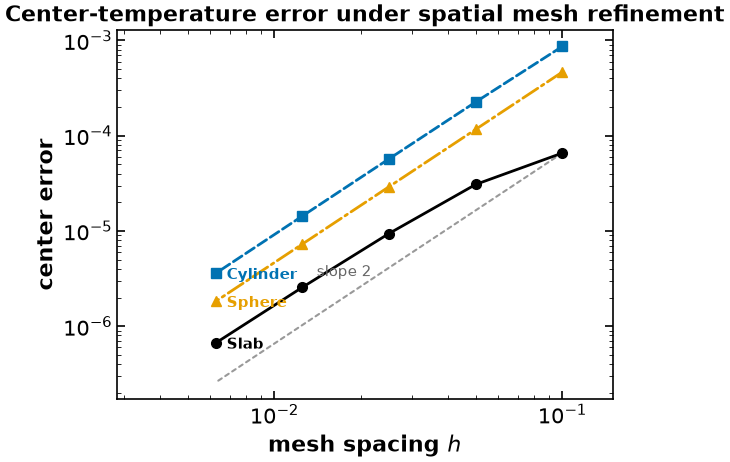
Three straight lines of slope 2, over four mesh halvings and more than two decades of error. That is what a consistent, correctly posed discretization looks like on a log-log plot, and it is the picture the dangling model cannot produce on the slab no matter how fine the mesh gets.
Reproducibility and archived figure data
The two figures printed in Lecture 7 are generated from committed numerical data, not from a
second implementation of this PDE. figures/results/heat-convergence.json stores the raw mesh-
refinement errors for all three geometries, the initial-guess experiment, and the expected
structural-diagnostics summary. figures/results/heat-slab-profile.json stores every profile and
analytical-series comparison for the slab, cylinder, and sphere; the handout uses the slab subset.
A maintainer re-renders either handout figure without Pyomo or IPOPT with:
python figures/render_from_notebook.py heat-convergence heat-slab-profileThe archived runs used Pyomo 6.10.1, IPOPT 3.13.2 (IDAES build with ma27), nfe_t=30, and
three Radau collocation points for the refinement experiment; the profile data use nfe_r=80,
nfe_t=50, and three Radau points. Exact iteration counts and timings are intentionally not used
as scientific evidence: they depend on the operating system, solver build, linear solver, and CPU.
The structural claims do not: the degree-of-freedom count, expected diagnostics cautions, initial-
guess invariance, and second-order convergence are the checks to reproduce.
The Correct Model, Geometry by Geometry
The builder is the same in all three cases. What changes is why each piece is correct.
Slab, 
The PDE is -- no singular term at all. We could legitimately write the
PDE row at and drop the symmetry condition; the slab is only “half” of a symmetric plate of
thickness , and is its midplane. We do not, for two reasons. scheme="CENTRAL" supplies
no second-derivative equation at either, so that row would need a one-sided stencil of its own;
and keeping the same skip-plus-symmetry structure for all three geometries means one code path, tested
three ways. So: skip the PDE at , impose with its defining equation.
Cylinder, 
Now the skip at is mandatory: cannot be evaluated there. The symmetry condition is doing real work -- it is the only equation that determines the axis temperature, and without a defining equation for the axis is unconstrained. Every interior row has , so the coefficient is finite everywhere it is used; it is large () at the first interior node, which is why the discrete operator is stiff near the axis and why an symmetry stencil is worth having.
Sphere, 
Identical structure, with . The weighting is stronger, so the near-center rows dominate the Jacobian even more -- which is also why the dangling model of the first table is least visibly wrong here. Nothing about the correct model changes.
In all three cases the count works out the same way, per time point: unknowns (the surface value is imposed), PDE rows at the interior nodes, and one center row. equations, unknowns, zero degrees of freedom -- which is what the DOF table above confirms.
# Production models: second-order symmetry stencil, fine mesh.
TIMES = [0.01, 0.05, 0.15, 0.5]

profile_rows = []
for s in [0, 1, 2]:
    m = build_fd(s=s, nfe_r=80, tf=max(TIMES), nfe_t=50, ncp=3)
    status = solve_model(m)
    rgrid = np.array(sorted(m.r))
    numeric_profiles = {}
    analytic_profiles = {}
    for tt in TIMES:
        # the collocation mesh contains every element boundary, and TIMES were
        # chosen to land on one; assert rather than silently interpolate
        assert tt in m.t, f"t = {tt} is not a mesh point"
        numeric_profiles[str(tt)] = [pyo.value(m.T[tt, r]) for r in rgrid]
        analytic_profiles[str(tt)] = analytic(s, tt, rgrid).tolist()
    err = max(
        np.max(np.abs(np.asarray(numeric_profiles[str(tt)]) - np.asarray(analytic_profiles[str(tt)])))
        for tt in TIMES if tt >= 0.05
    )
    profile_rows.append({
        "shape_index": s,
        "geometry": GEOMETRY[s],
        "status": str(status),
        "r": rgrid.tolist(),
        "numeric_profiles": numeric_profiles,
        "analytic_profiles": analytic_profiles,
        "max_abs_error_for_fo_ge_0_05": float(err),
    })
    print(f"{GEOMETRY[s]:9s} status = {status},  max |numeric - series| over r for Fo >= 0.05: {err:.2e}")

profile_results = {
    "times": TIMES,
    "nfe_r": 80,
    "nfe_t": 50,
    "ncp": 3,
    "geometries": profile_rows,
}
helper.save_results(
    "heat-slab-profile",
    profile_results,
    notebook="notebooks/3-dev/heat_conduction_pde.ipynb",
    description=(
        "Raw temperature profiles for the slab, cylinder and sphere, calculated "
        "with the shipped finite-difference spatial discretization and Radau "
        "collocation in time. The handout shows the slab subset; this archive retains "
        "all three geometries and the analytical-series comparison."
    ),
    solver="Ipopt 3.13.2 (IDAES build, linear solver ma27); Pyomo 6.10.1",
)
results = profile_results
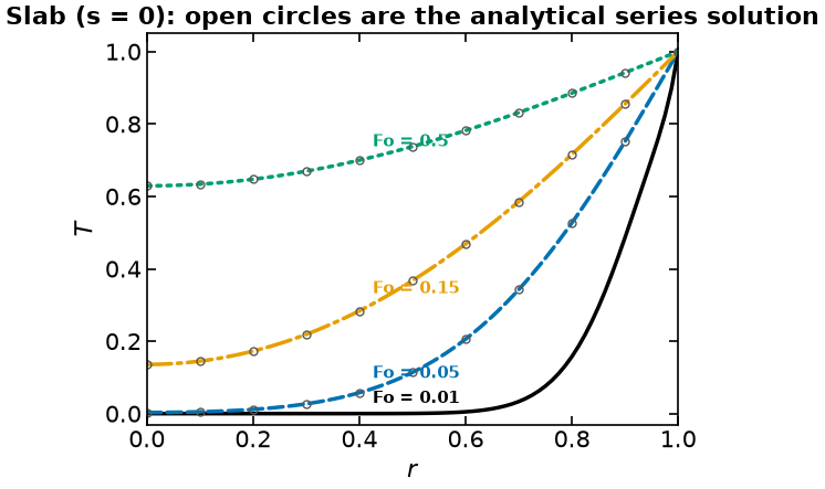
Slab status = optimal, max |numeric - series| over r for Fo >= 0.05: 4.26e-05
Cylinder status = optimal, max |numeric - series| over r for Fo >= 0.05: 8.26e-05
Sphere    status = optimal,  max |numeric - series| over r for Fo >= 0.05: 1.34e-04
[helper] wrote figures/results/heat-slab-profile.json
fig, axes = plt.subplots(1, 3, figsize=(13, 4.6), sharey=True)

for ax, row in zip(axes, results["geometries"]):
    rgrid = np.asarray(row["r"], dtype=float)
    for tt in results["times"]:
        key = str(tt)
        (line,) = ax.plot(rgrid, row["numeric_profiles"][key], lw=2.5)
        # direct labelling: a legend keyed only by colour dies in black and white
        j = int(0.42 * len(rgrid))
        ax.annotate(f"Fo = {tt:g}", xy=(rgrid[j], row["numeric_profiles"][key][j]),
                    xytext=(0, 7), textcoords="offset points",
                    fontsize=11, color=line.get_color(), fontweight="bold")
    # series solution, as sparse open markers, for the two well-resolved times
    for tt in results["times"][1:]:
        key = str(tt)
        ax.plot(rgrid[::8], np.asarray(row["analytic_profiles"][key])[::8], ls="none", marker="o",
                mfc="none", mec="0.35", ms=5, mew=1.0)
    ax.set_xlabel("$r$")
    ax.set_title(f"{row['geometry']}  (s = {row['shape_index']})")
    ax.set_xlim(0, 1)
    ax.set_ylim(-0.03, 1.05)

axes[0].set_ylabel("$T$")
fig.suptitle("Temperature profiles: open circles are the analytical series solution", y=1.02)
plt.show()
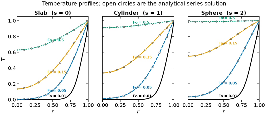
The lecture handout carries the slab profile and the convergence plot above. The slab is the geometry where the dangling-variable defect is loud, so it is the one worth printing. The cylinder and sphere are on this page only — see the three-panel figure above.
fig, ax = plt.subplots(figsize=(6.2, 4.6))

slab = results["geometries"][0]
rgrid = np.asarray(slab["r"], dtype=float)
for tt in results["times"]:
    key = str(tt)
    (line,) = ax.plot(rgrid, slab["numeric_profiles"][key], lw=2.5)
    j = int(0.42 * len(rgrid))
    ax.annotate(f"Fo = {tt:g}", xy=(rgrid[j], slab["numeric_profiles"][key][j]),
                xytext=(0, 7), textcoords="offset points",
                fontsize=11, color=line.get_color(), fontweight="bold")
for tt in results["times"][1:]:
    key = str(tt)
    ax.plot(rgrid[::8], np.asarray(slab["analytic_profiles"][key])[::8], ls="none", marker="o",
            mfc="none", mec="0.35", ms=5, mew=1.0)
ax.set_xlabel("$r$")
ax.set_ylabel("$T$")
ax.set_title("Slab (s = 0): open circles are the analytical series solution")
ax.set_xlim(0, 1)
ax.set_ylim(-0.03, 1.05)

# Write media/figures/heat-slab-profile.{png,pdf} for the lecture handout.
helper.save_figure(fig, "heat-slab-profile")
plt.show()
[helper] wrote media/figures/heat-slab-profile.png and .pdf
At a fixed Fourier number the sphere is furthest along and the slab is furthest behind. That is the surface-to-volume ratio: per unit volume, a sphere presents of surface, a cylinder , a slab . The shape index is doing exactly that bookkeeping, and it is the reason alone is not enough to say “how hot is it inside” without also saying which shape you meant.
fig, ax = plt.subplots(figsize=(6.2, 4.6))

for s in [0, 1, 2]:
    m = build_fd(s=s, nfe_r=80, tf=0.5, nfe_t=50, ncp=3)
    solve_model(m)
    tgrid = np.array(sorted(m.t))
    Tc = np.array([pyo.value(m.T[t, 0]) for t in tgrid])
    (line,) = ax.plot(tgrid, Tc, lw=2.5)
    frac = {0: 0.62, 1: 0.34, 2: 0.26}[s]  # keep the three labels off each other
    k = int(frac * len(tgrid))
    ax.annotate(GEOMETRY[s], xy=(tgrid[k], Tc[k]), xytext=(6, -18),
                textcoords="offset points", fontsize=12,
                color=line.get_color(), fontweight="bold")

ax.set_xlabel("Fourier number  $\\mathrm{Fo} = \\alpha t / R^2$")
ax.set_ylabel("center temperature $T(t, 0)$")
ax.set_xlim(0, 0.5)
ax.set_ylim(-0.03, 1.03)
ax.set_title("Heating from a step change at the surface")
plt.show()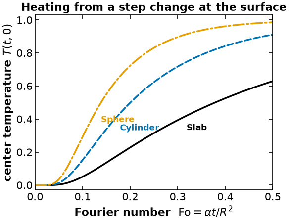
The Finite Volume Alternative
Everything above was finite difference. It is worth building the finite volume version of the same problem, because it makes a structural point that no amount of care with stencils can:
In the finite volume formulation the symmetry condition at is not a boundary condition at all. It is a consequence of the geometry, and there is nothing to forget.
Place shells with faces at , , and unknowns at the cell centers. The balance on shell is the discrete form of the integral law from earlier,
For the innermost shell, and therefore for : the inner face has no area, so no heat can cross it. For the slab, makes , and we set the inner flux to zero by symmetry -- one line, and the only geometry-specific line in the model.
At the outer face of the last shell the temperature is known, and the half-cell distance from the center of that shell to the surface is , so the flux is .
Note also that there is no DerivativeVar in space at all. The method of lines is explicit here: the
only ContinuousSet is time.
def build_fv(s, ncells, tf=0.5, nfe_t=30, ncp=3):
    """Finite volume discretization of the same problem.

    Shells of equal thickness h = 1/ncells, unknowns at cell centers, fluxes at faces.
    Conservative by construction, and the symmetry condition at r = 0 is structural.
    """
    h = 1.0 / ncells
    faces = np.linspace(0.0, 1.0, ncells + 1)
    centers = 0.5 * (faces[:-1] + faces[1:])
    area = faces**s                                     # A = r^s at each face
    vol = (faces[1:] ** (s + 1) - faces[:-1] ** (s + 1)) / (s + 1)

    m = pyo.ConcreteModel()
    m.t = dae.ContinuousSet(bounds=(0, tf))
    m.c = pyo.RangeSet(0, ncells - 1)                   # cell index; NOT a ContinuousSet
    m.T = pyo.Var(m.t, m.c, initialize=0.0)
    m.dTdt = dae.DerivativeVar(m.T, wrt=m.t)

    @m.Constraint(m.t, m.c)
    def shell(m, t, i):
        if t == 0:
            return pyo.Constraint.Skip
        if i == 0:
            flux_in = 0.0                               # zero face area (s>0) or symmetry (s=0)
        else:
            flux_in = area[i] * (m.T[t, i] - m.T[t, i - 1]) / h
        if i == ncells - 1:
            flux_out = area[i + 1] * (1.0 - m.T[t, i]) / (h / 2)   # bath at r = 1
        else:
            flux_out = area[i + 1] * (m.T[t, i + 1] - m.T[t, i]) / h
        return vol[i] * m.dTdt[t, i] == flux_out - flux_in

    @m.Constraint(m.c)
    def ic(m, i):
        return m.T[0, i] == 0

    pyo.TransformationFactory("dae.collocation").apply_to(
        m, wrt=m.t, nfe=nfe_t, ncp=ncp, scheme="LAGRANGE-RADAU"
    )
    m.obj = pyo.Objective(expr=0.0)
    m.centers = centers
    return m
NC_LIST = [10, 20, 40, 80]
print(f"{'geometry':10s} {'DOF':>5s} " + "".join(f"{'N='+str(n):>12s}" for n in NC_LIST) + f"{'order':>9s}")
fv_conv = {}
for s in [0, 1, 2]:
errs = []
for n in NC_LIST:
m = build_fv(s=s, ncells=n)
solve_model(m)
# compare at the first cell center, r = h/2
errs.append(abs(pyo.value(m.T[0.5, 0]) - analytic(s, 0.5, m.centers[0])[0]))
fv_conv[s] = np.array(errs)
rep = build_model_size_report(build_fv(s=s, ncells=40)).activated
order = np.log2(errs[-2] / errs[-1])
print(f"{GEOMETRY[s]:10s} {rep['variables'] - rep['constraints']:5d} "
+ "".join(f"{v:12.3e}" for v in errs) + f"{order:9.2f}")geometry DOF N=10 N=20 N=40 N=80 order
Slab 0 1.318e-03 3.299e-04 8.251e-05 2.063e-05 2.00
Cylinder 0 9.179e-04 2.294e-04 5.734e-05 1.433e-05 2.00
Sphere 0 3.672e-04 9.172e-05 2.293e-05 5.734e-06 2.00
Zero degrees of freedom in every geometry, second-order convergence, and no symmetry constraint anywhere in the model. The Diagnostics Toolbox says the same thing structurally.
DiagnosticsToolbox(build_fv(s=1, ncells=8, nfe_t=4)).report_structural_issues()====================================================================================
Model Statistics
Activated Blocks: 1 (Deactivated: 0)
Free Variables in Activated Constraints: 200 (External: 0)
Free Variables with only lower bounds: 0
Free Variables with only upper bounds: 0
Free Variables with upper and lower bounds: 0
Fixed Variables in Activated Constraints: 0 (External: 0)
Activated Equality Constraints: 200 (Deactivated: 0)
Activated Inequality Constraints: 0 (Deactivated: 0)
Activated Objectives: 1 (Deactivated: 0)
------------------------------------------------------------------------------------
0 WARNINGS
No warnings found!
------------------------------------------------------------------------------------
1 Cautions
Caution: 8 unused variables (0 fixed)
------------------------------------------------------------------------------------
Suggested next steps:
Try to initialize/solve your model and then call report_numerical_issues()
====================================================================================
Zero warnings again, and this time a single caution: the 8 unused variables are at , one per cell, which Radau collocation never references. There is no “fixed to 0” caution, because there is nothing to fix -- and that is the argument for finite volume in one line. Not that it is more accurate (on this uniform mesh it is not dramatically so), but that the condition we spent the first half of this notebook getting right cannot be gotten wrong: the inner face of the first shell has zero area, so no heat can cross it, structurally and on every mesh.
The price is that a finite volume model is yours to write. Pyomo.dae will not build it for you,
you do not get a DerivativeVar to inspect, and the cell-center unknowns do not sit on the boundary,
so reporting a surface value takes an extra half-cell extrapolation. Which is the right trade depends
on the problem, and that is the point of knowing all three families.
The mistakes move with the method. Finite volume cannot lose the symmetry condition, but it has its own short list -- and, symmetrically with the first table, its worst failure is the one the slab cannot see.
Alternative Finite Volume Discretizations, and What They Do
Same convention as the first table: these were measured, not reasoned about, and none of them ships as
a runnable option above. Conditions are , nfe_t=30, ncp=3 Radau, IPOPT
3.13.2 with ma27, and cells. The error is taken at the first cell center,
, against the series solution evaluated there; “order” is of the ratio of the last two.
| Alternative discretization | Modeling issue | Failure evidence (measured) |
|---|---|---|
| Evaluate the face areas at the cell center, , instead of at the faces | Not conservative. The flux leaving cell is no longer identically the flux entering cell , so the sum over cells stops telescoping -- the one property finite volume exists to provide. For it is not even consistent. | Slab unaffected ( either way, so the bug is invisible at ). Cylinder error plateaus at 0.2824, 0.2820, 0.2819, 0.2819 -- observed order 0.00. Sphere 0.3890, 0.3738, 0.3654, 0.3610 -- observed order 0.02. Every solve returned optimal. 🔴 The mirror image of the finite difference trap: loud on the cylinder and sphere, silent on the slab. |
| Lumped cell volume instead of the exact shell volume | First-order mass matrix. The volume multiplies ; approximating it to degrades the whole scheme even though it stays conservative, square and stable. Tempting because it is one fewer line. | Slab unaffected (the volume is exact there). Cylinder 5.22e-2, 2.53e-2, 1.24e-2, 6.14e-3 -- observed order 1.02. Sphere 2.99e-2, 1.20e-2, 5.33e-3, 2.50e-3 -- observed order 1.09. Against order 2.00 for the shipped model. |
| Outer boundary flux over the full cell width instead of the half cell | Wrong distance at the Dirichlet face. The last unknown sits at a cell center, a distance from the surface. Using halves the surface flux and makes a first-order boundary error the accuracy bottleneck -- the finite volume version of an under-resolved boundary row. | Order falls to 1.00 in all three geometries: slab 4.51e-2 5.71e-3, cylinder 2.83e-2 3.26e-3, sphere 9.04e-3 9.15e-4 over . |
| Node-centered layout with an explicit symmetry boundary condition at (i.e. put an unknown on the axis) | Reintroduces the Neumann condition that cell-centered finite volume removes -- and with it the dangling-variable failure mode in full. | See the finite difference table above; this is that table. |
| ✅ Shipped: cell-centered, face areas at the faces, exact shell volumes, half-cell surface flux | Conservative by construction; the symmetry condition is structural, not written. | DOF = 0 in all three geometries, 0 warnings from report_structural_issues(), observed order 2.00 everywhere, and no symmetry constraint anywhere in the model. |
Take-Home Messages
Nondimensionalize first. Three geometries, any material, any size and any temperature pair reduce to one equation in one parameter , with the Fourier number as the clock.
The method of lines is a decision, not a syntax. Discretizing space first is what lets you hand the time direction to Lecture 7’s collocation machinery and concentrate on the spatial operator, where the physics lives.
Finite difference, finite volume and finite element differ in what they reproduce exactly -- the Taylor series, the integral balance, or a weighted residual. Reach for FV when conservation or an interface matters, FE when the geometry or the accuracy demands it, FD when neither does.
🔴 A Neumann boundary condition written on a
DerivativeVarmay constrain nothing.CENTRALfinite differences and Radau collocation both leave the derivative at the left endpoint of the domain with no defining equation. Writingm.dTdr[t, 0] == 0and stopping there assigns a value to a dangling variable, and the center temperature is unconstrained. Write the defining equation too.optimalis notcorrect. Every failure in the two tables above terminated cleanly, several of them with plausible-looking numbers. Three things catch this class of defect: a degree-of-freedom count -- a simulation must have zero --report_structural_issues(), which says which variables are loose rather than how many, and mesh refinement, which turns a structural defect into a visible plateau. Do all three.Run the diagnostics before you run the solver.
report_structural_issues()needs no solution and no initialization; it costs seconds and it reads the incidence pattern you cannot read by eye. Learn what cautions your model should emit, so that a new one means something.Test on the geometry where the bug is loud. The finite difference defect was obvious in the slab and nearly invisible in the sphere; the finite volume defect is the other way round. A model verified only on the forgiving case is not verified.
Try It Yourself
Predict, before running it, which endpoint loses its defining equation under
scheme="BACKWARD"and what that breaks inbuild_fd. Check your answer withstencil_coverage("BACKWARD")-- and then say what one-sided row you would owe the model to repair it.Replace
dae.finite_differencein space withdae.collocationin a copy ofbuild_fdand confirm, with the toolbox rather than by eye, that the derivative at still needs a defining equation of your own.Add a Robin (convective) boundary condition at the surface, , where is the Biot number. Which endpoint does
CENTRALleave undefined now, and what does that imply about which one-sided stencil you owe the model? Recover the results above as .Grade the mesh toward so the short-time boundary layer is resolved, and redo the comparison.
ContinuousSet(initialize=[...])accepts an explicit list of points.Reproduce one row of either table for yourself in a scratch copy of the builder -- then delete it. Confirming a documented failure mode is worth an hour; leaving a runnable broken model in a notebook someone else will copy is not.