Local Optimality Conditions

Reference Section 4.2 in Biegler (2010)

Unconstrained comparison¶

For twice continuously differentiable objectives, a local unconstrained minimum has zero gradient and positive-semidefinite Hessian. These are necessary conditions; they do not classify every stationary point. The definitions, derivative tests and proofs have their existing home in Unconstrained Optimality Conditions. Here the feasible neighborhood and constraint reactions change the test.

Balance of Forces Interpretation¶

Here is a helpful handout.

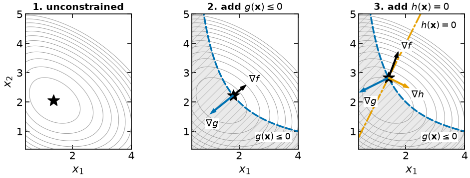
Consider $\min f(\mathbf{x})$ subject to $g(\mathbf{x})\le0$. The objective is a landscape; its downhill force is $-\nabla f$. The fence force is $-u\nabla g$, with $u\ge0$, pointing toward the feasible side.

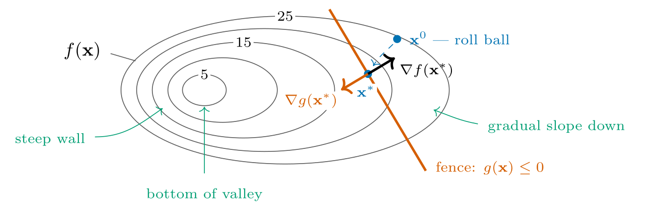
The drawn arrows are gradients, pointing toward increasing values. At a regular constrained minimum with an active pushing fence,

The objective contour is tangent to the fence. Opposite gradient directions do not require equal lengths: the multiplier supplies the scale. Rescaling a constraint changes the numerical multiplier, so raw arrow lengths are not force magnitudes.

Source: Biegler (2010), Figures 4.5–4.6, pp.68–69. The handout and website use this same prepared drawing.

An equality $h(\mathbf{x})=0$ acts as a rail. Its force $-v\nabla h$ can point either way, because $v$ is unrestricted.

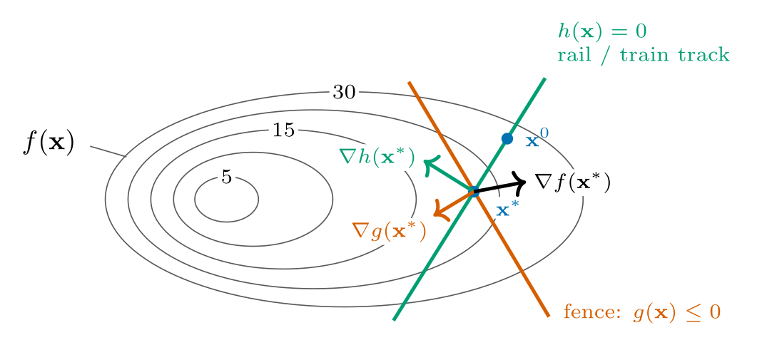
Balance is $\nabla f+u\nabla g+v\nabla h=0$. For this illustrative drawing the normalized gradients are approximately

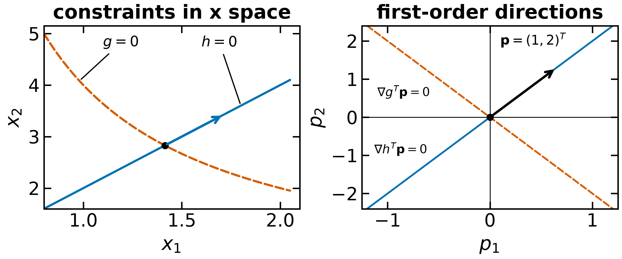
They give $u\approx0.76265>0$, $v\approx0.38634$. The direction $\mathbf p=(0.5300,0.8480)^T$ is tangent to the rail, enters the feasible side of the fence, and raises the objective to first order. Its negative crosses the fence. Thus there is feasible motion, but no nonzero critical direction at this intersection. “No allowable directions” in a curvature discussion refers to the critical cone, not all feasible motion.

For the displayed rounded vectors, the equality tangent space is one-dimensional: every tangent vector is $\mathbf p=t(0.5300,0.8480)^T$, $t\in\mathbb R$. The exact dot products of these supplied decimals are

The linearized inequality therefore requires $t\ge0$, and zero first-order objective change then requires $t=0$. This establishes the whole critical cone $\{0\}$ rather than testing only one direction. These conclusions describe the prepared drawing; the derivatives of the later log-model are calculated independently.

Removing the rail permits a downhill direction along the fence toward its tangency minimum. For example, $\mathbf q=(-0.5125,0.8587)^T$ has $\nabla g^T\mathbf q=0$ and $\nabla f^T\mathbf q=-0.34372718<0$. But $\nabla h^T\mathbf q=0.889711\ne0$, so the rail excludes this descent direction. Source: Biegler (2010), Figure 4.7 and Eq. (4.9), pp.70–71. The later numerical example uses its own objective and gradients; these normalized drawing vectors are not substituted into that model.

Karush-Kuhn-Tucker (KKT) necessary conditions¶

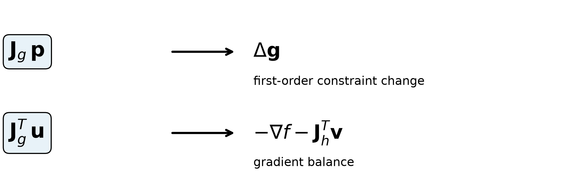
Use row-oriented Jacobians $\mathbf J_g\in\mathbb R^{r\times n}$ and $\mathbf J_h\in\mathbb R^{m\times n}$ and

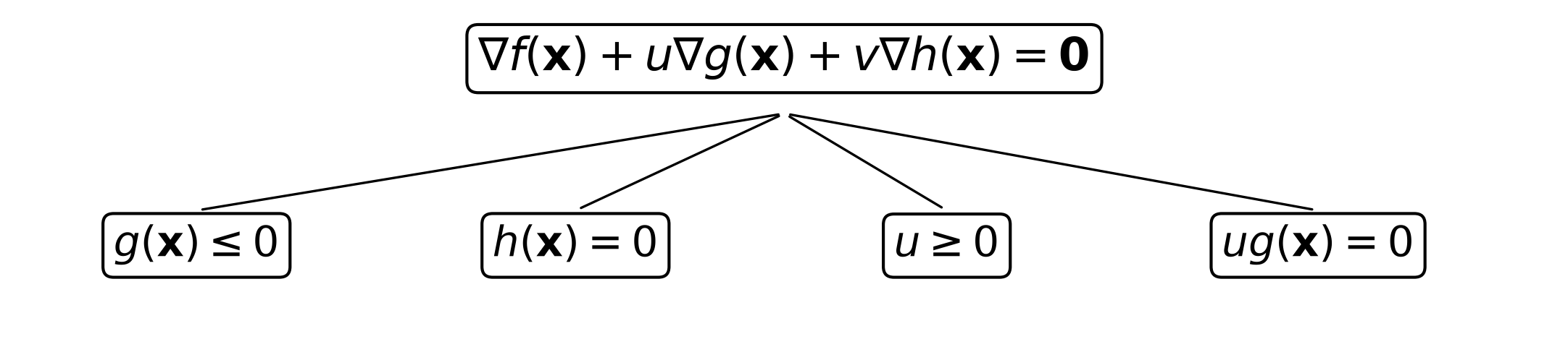
Assume $C^1$ data on an open neighborhood of a feasible local minimum. If LICQ holds there, the following necessary multiplier conditions apply:

Evaluate these at the candidate. Equality multipliers have no sign restriction. Dot-product complementarity $\mathbf g^T\mathbf u=0$ is equivalent to the component conditions because every summand is nonpositive. The prepared product-vector diagram compares nonpositive terms with a zero vector. If any term is strictly negative, no other nonpositive term can cancel it to make the sum zero.

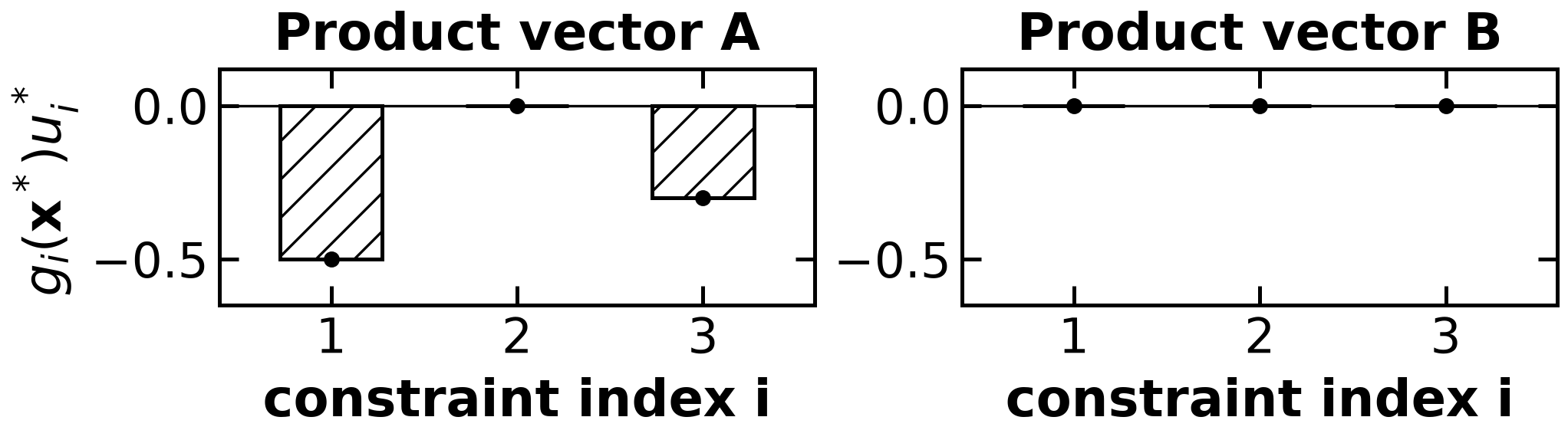
Inactive constraints have $g_i<0$, hence $u_i=0$. Active constraints have $g_i=0$ and may have a positive multiplier (strongly active) or zero multiplier (weakly active).

Regularity is a hypothesis. LICQ means the equality gradients and active inequality gradients are linearly independent. It is one sufficient qualification for the first-order necessary conditions. For $\min x$ subject to $x^2=0$, the only feasible point is a strict global minimum, but $1+v(2x)=0$ cannot hold at zero for any multiplier. The constraint gradient is zero. See Constraint Qualifications for the full theory.

Feasible and critical directions differ. The linearized feasible cone imposes $\mathbf J_h\mathbf p=0$ and $\nabla g_i^T\mathbf p\le0$ on active inequalities. At a KKT point,

Critical directions have zero first-order objective change. Since every term on the right is nonnegative, they are exactly the directions satisfying

A positive multiplier does not prevent every feasible inward move; it makes that move raise the objective to first order. Such a direction is not critical. These are first-order tangent tests; nonlinear constraints need not remain feasible along an entire straight step.

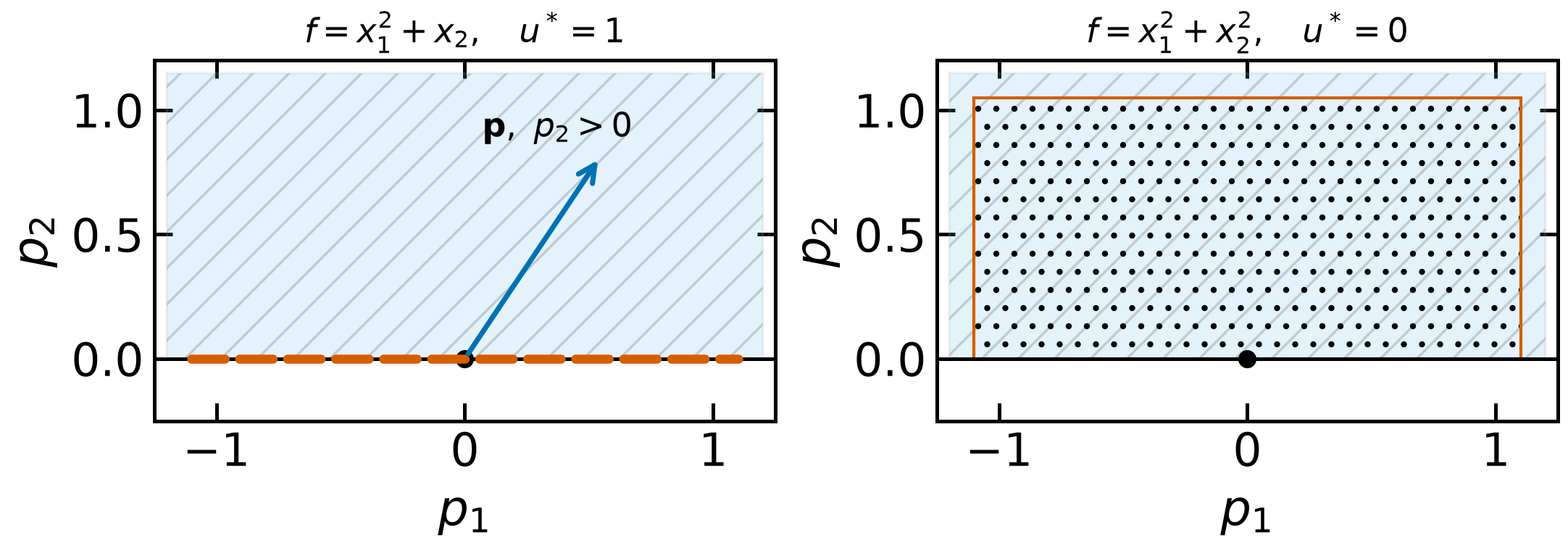
For $g=-x_2$ at the origin, $f=x_1^2+x_2$ has $u=1$ and critical directions $p_2=0$. Its feasible directions with $p_2>0$ already raise the objective. For $f=x_1^2+x_2^2$, $u=0$ and every linearized feasible direction $p_2\ge0$ is critical.

With $C^2$ data on an open neighborhood and LICQ at a local minimum, second-order necessity gives

Together with KKT, strict positivity on every nonzero critical direction is sufficient for a strict local minimum. The two examples satisfy it on their respective cones. If the critical cone is $\{0\}$, the strict condition is vacuous; feasible noncritical directions are controlled by their positive first-order change. Full theorem/proof material has its existing home in Second-Order Conditions.

Sources: Biegler (2010), Eqs. (4.9)–(4.12), pp.70–71; Theorems 4.14–4.15, pp.77–78; critical cone in §4.3.3, p.79; Theorems 4.17–4.18, pp.80–81. The constraint-qualification counterexample follows directly from its singleton feasible set and zero constraint derivative.

Kinematic Interpretation via Example¶

Consider the following two dimensional optimization problem:

Define Function for Visualization¶

Define function to solve optimization problem with Pyomo¶

Three constraint cases¶

The three solves below feed the shared prepared figure after Take 3. The complete visualization, plotting implementation and archived results have one source in this notebook.

Take 1: Unconstrained¶

Take 2. With $g(\mathbf{x}) \leq 0$¶

Take 3. With $g(\mathbf{x}) \leq 0$ and $h(\mathbf{x}) = 0$¶

Shared figure from the three notebook solves¶

The same archived primal points, gradients and objective grid produce the handout and website figure. The plotting cell runs without a solver when those results are supplied.

Hatching in the three-panel numerical picture marks $g(\mathbf x)>0$, the infeasible side. The label $g(\mathbf x)\le0$ names the imposed inequality; its feasible side is above the hyperbola. The equality rail is the dash-dot line in Take 3.

Discussion¶

Why are the gradient vectors not the same length? I thought the forces were balanced...

Analysis without Constraints¶

For the unconstrained problem, stationarity requires

Numerically, $\mathbf{x}^*=(1.3475,\,2.0470)$ and $f(\mathbf{x}^*)=-0.8742$. Moreover,

so $\mathbf{x}^*$ is a strict local minimizer.

Analysis with Constraints¶

KKT system and exact certificate¶

For the constrained problem, define

The concrete KKT system is

with $x_1,x_2>0$ and $v\in\mathbb R$. Products and reciprocals make the stationarity equations nonlinear. Complementarity supplies separate active-state branches, while domain, primal feasibility and multiplier signs remain mandatory checks on every root.

The exact point is $(\sqrt2,2\sqrt2)^T$. Solving the KKT conditions gives the rounded values

with $g(\mathbf{x}^*)=0$, $h(\mathbf{x}^*)=0$, and $f(\mathbf{x}^*)=0.1579$. The Lagrangian Hessian is

The exact multipliers are $u^*=(17-9\sqrt2)/4>0$ and $v^*=(5/2)(\sqrt2-1)$. The active inequality and equality gradients are independent. Since the inequality multiplier is positive, a critical direction must be tangent to both constraints; the critical cone is $\{0\}$, so the second-order sufficient condition is satisfied vacuously. Feasible motion still exists: $\mathbf p=(1,2)^T$ is tangent to the equality and enters the inequality interior, but raises the objective to first order.

This particular example also admits a global certificate. On its positive log domain, $4-x_1x_2\le0$ is equivalent to $4/x_1-x_2\le0$, a convex inequality; its second derivative in $x_1$ is $8/x_1^3>0$. The equality is affine, and the objective Hessian is positive definite throughout the domain: its diagonal entries exceed 2 and 3, with off-diagonal entry 1, so its determinant exceeds 5. The problem therefore has a convex feasible set and a strictly convex objective even though the original product constraint function is not convex. The local minimum is the unique global minimum. This illustrates the representation distinction in Convexity Revisited, rather than applying a failed structural test as a converse.

Sources: Biegler (2010), Eqs. (4.16)–(4.24), p.72; Theorem 4.3, p.65, and Theorem 4.18, p.81. The equivalent-constraint/global certificate and exact multipliers are independently derived from the displayed model. Objective-value source correction: the displayed model has constant +9, yielding approximately -0.874224 without constraints and 0.157862 with both constraints. The book’s -2.8742 and -1.8421 are two units lower and correspond to replacing that constant by +7. The additive constant changes values but not gradients, minimizers, multipliers or curvature. We keep the displayed +9 model and its independently evaluated values.

Active-branch and Hessian details for this same model¶

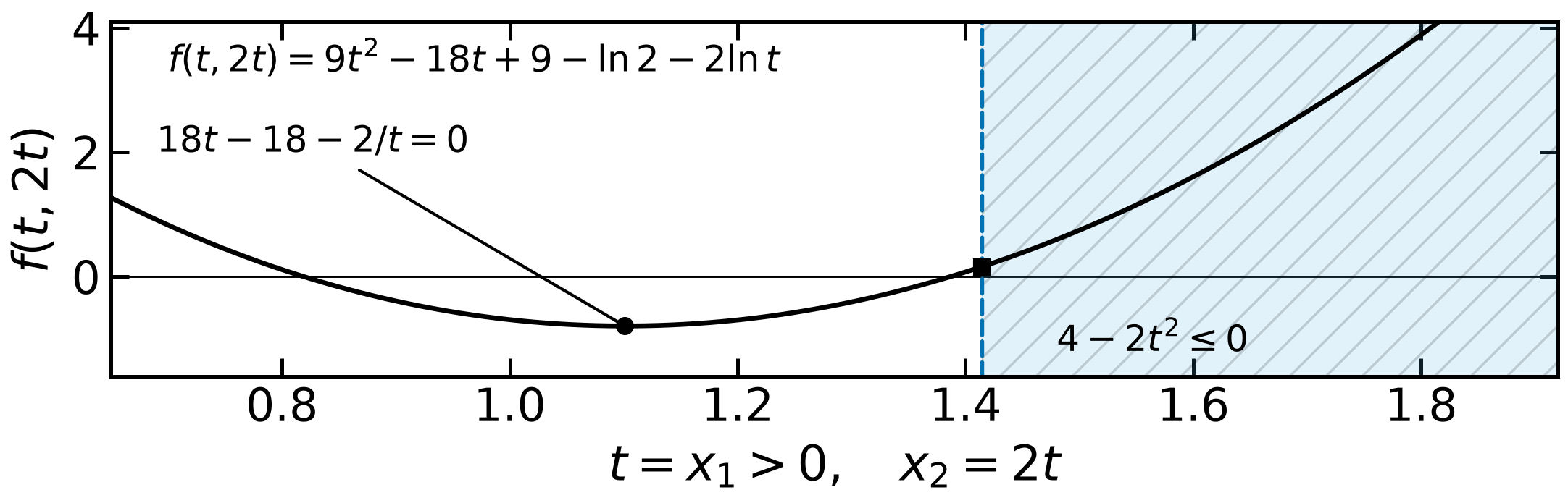
If the equality is retained but the inequality is assumed slack, set $u=0$ and $x_2=2x_1$. The restricted objective is

Stationarity gives $18x_1-18-2/x_1=0$, or $9x_1^2-9x_1-1=0$. Its positive root is $(9+\sqrt{117})/18\approx1.100925$, with $x_2\approx2.201850$. But $g=4-2x_1^2\approx1.575927>0$, so this branch is infeasible. The active branch instead enforces $4-2x_1^2=0$, and the positive domain selects the exact point derived above. A root is accepted only after domain, primal feasibility, multiplier sign and complementarity checks.

The Lagrangian Hessian is a sum of scalar-component Hessians,

At the exact constrained point, the diagonal entries are 2.5 and 3.125, and the off-diagonal is $1-u^*=(9\sqrt2-13)/4\approx-0.068019$. Biegler Eq.(4.24) p.72 prints a positive off-diagonal. The errata fixes the diagonal signs but leaves that further sign error. The critical-direction matrix

has determinant $4\sqrt2$, so its null space is zero. It describes directions tangent to the equality and the positively weighted active inequality. It does not describe every feasible direction: $(1,2)^T$ is an inward feasible rail direction and increases the objective to first order.

Printed orientation discrepancy. Biegler Eq.(4.9) p.70 uses transposed vector-constraint gradients, while Eqs.(4.17)–(4.18) p.72 use columns for the same stationarity components. The course consistently defines $\mathbf J_g$ with constraint rows ($r\times n$), so $\mathbf J_g\mathbf p$ is a constraint-change vector and $\mathbf J_g^T\mathbf u$ is an $n$-component gradient contribution. A single scalar-constraint gradient is a column. This resolves the dimensions without adopting two definitions of the same symbol.

Sources: Biegler Eqs.(4.13), (4.16)–(4.25), pp.71–72, with the displayed positive-domain substitutions and exact derivatives independently checked. The complete multiplier-sensitivity and strong/weak reference is Analysis of KKT Conditions.