Analysis of KKT Conditions

Reference: Biegler (2010), Chapter 4, §4.3, pp.72–74; Rockafellar (1993), Lagrange Multipliers and Optimality, §9, pp.224–225. The log-model and its nonlinear KKT system have their complete home in Local Optimality Conditions. Constraint Qualifications develops multiplier existence/uniqueness and the link to actual feasible directions.

Active Sets¶

Let $D\subset\mathbb R^n$ be open, with $f:D\to\mathbb R$, $\mathbf g:D\to\mathbb R^r$, and $\mathbf h:D\to\mathbb R^m$. The inequalities are componentwise.

For $\min f(\mathbf{x})$ subject to $\mathbf{g}(\mathbf{x})\le\mathbf{0}$ and $\mathbf{h}(\mathbf{x})=\mathbf{0}$, define equality indices $\mathcal{E}=\{1,\ldots,m\}$ and inequality indices $\mathcal{I}=\{1,\ldots,r\}$. The active inequality index set at a feasible point is

If both types are collected into one set, use distinct constraint labels:

Equality $h_1$ and inequality $g_1$ are different constraints, even though their component indices are both 1. The inactive inequality indices are $\mathcal{I}\setminus\mathcal{A}_I$, rather than a difference with untagged equality indices. All equalities belong to the combined active set at every feasible point.

Why an inactive constraint drops out locally. Suppose $g_i(\mathbf{x}^*)<0$ and $g_i$ is continuous. There is $\rho_i>0$ such that $g_i(\mathbf x)<0$ for every $\mathbf x\in\mathcal B(\mathbf x^*,\rho_i)\subset D$, where $\mathcal B(\mathbf x^*,\rho_i)=\{\mathbf x:\|\mathbf x-\mathbf x^*\|<\rho_i\}$. For finitely many inactive inequalities, take the intersection of these neighborhoods. Removing them leaves exactly the same feasible comparisons in that neighborhood. Their KKT multipliers are zero by complementarity, so they contribute nothing to gradient balance either. This is a local argument, not permission to remove them from the optimization model.

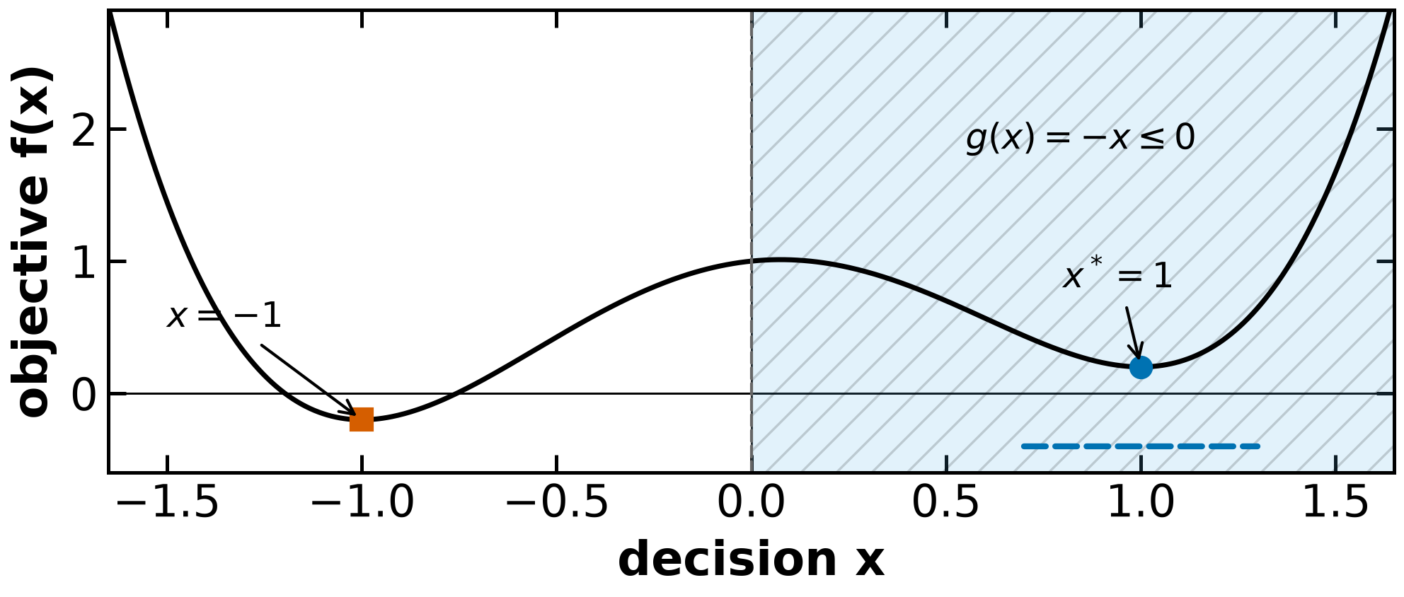
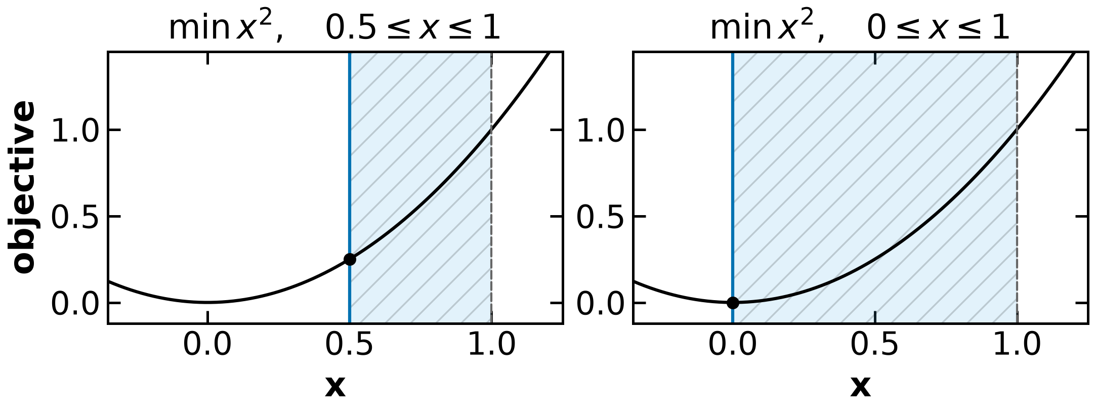
The prepared example uses $f(x)=(x^2-1)^2+0.1(3x-x^3)$ and $g=-x\le0$. Its derivative is $(x^2-1)(4x-0.3)$. At $x=1$, $f''=7.4>0$, $g=-1$ and $f=0.2$. Every point in $(0.7,1.3)$ satisfies the inequality, so it is irrelevant to that local test. Removing it globally admits the other strict local minimum $x=-1$, with value -0.2. A constraint that is inactive at the current solution can still exclude a better distant solution.

Source: Biegler p.72 for the active/local characterization; explicit index spaces, continuity proof and polynomial example are independently specified here.

Sensitivity Analysis¶

A smooth local branch and a moving constraint¶

Choose $\hat\imath\in\mathcal{A}_I(\mathbf{x}^*)$ and replace just one inequality by

Positive $\epsilon$ tightens the right-hand side to $-\epsilon$; negative $\epsilon$ relaxes it. Let $\mathbf{x}^{\epsilon}$ be a nearby local minimizer branch, with $\mathbf{x}^0=\mathbf{x}^*$, and put $V(\epsilon)=f(\mathbf{x}^{\epsilon})$. This is a local branch value. It need not select the global minimum for every perturbed problem.

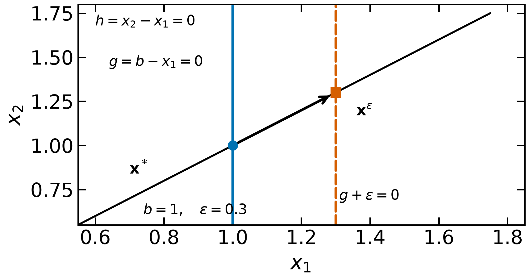
The drawing uses $f=x_1^2+x_2^2$, $g=b-x_1\le0$, $h=x_2-x_1=0$, and $b=1$. The exact solution branch is $\mathbf{x}^{\epsilon}=(b+\epsilon,b+\epsilon)^T$ for $b+\epsilon>0$. It has $V(\epsilon)=2(b+\epsilon)^2$, $V'(0)=4b$, inequality multiplier $u^*=4b$ and equality multiplier $v^*=-2b$.

Hypotheses for the following Taylor proof. The data are continuously differentiable; $\mathbf{x}^{\epsilon}$ is differentiable at zero; there exists $\delta>0$ such that the same inequalities remain active for every $|\epsilon|<\delta$. Thus

Taylor remainders are therefore $o(\epsilon)$, meaning their norm divided by $|\epsilon|$ tends to zero. The active-set statement alone does not justify dividing an uncontrolled approximation by $\epsilon$.

1. Equalities are satisfied at both points:

2. Every unperturbed active inequality is still zero:

3. The selected one stays active at its changed bound:

Full objective substitution¶

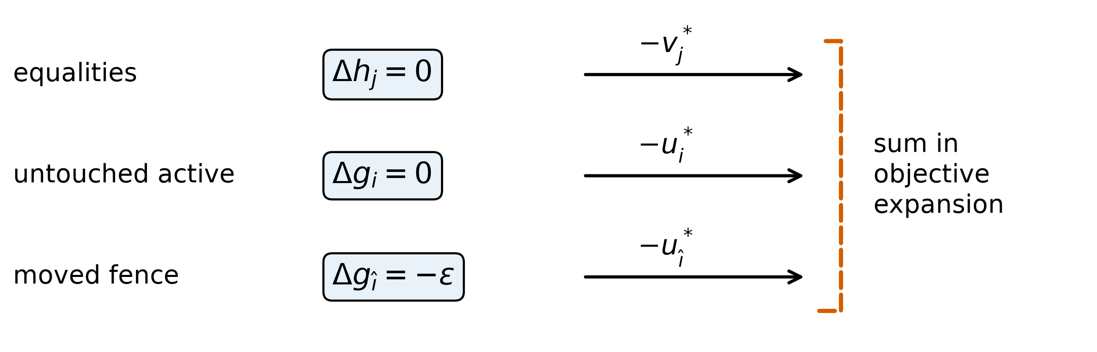
At the unperturbed KKT point,

Use the objective expansion and substitute this identity:

All equality differences vanish. Inactive inequalities have $u_i^*=0$. Untouched active inequalities have zero constraint difference. The selected constraint has difference $-\epsilon$, and its contribution is $-u_{\hat\imath}^*(-\epsilon)$. Hence

This is the sign convention for $g+\epsilon\le0$. If instead the constraint is written $g\le b$, increasing $b$ relaxes it and the derivative with respect to $b$ is $-u^*$. For an equality written $h+\eta=0$, the same substitution gives $\partial V/\partial\eta=v^*$. With a differentiable multi-parameter branch,

Rescaling $g$ to $c g$, $c>0$, changes the multiplier to $u/c$. Its units and numerical magnitude depend on the constraint’s scaling; the product of multiplier and the corresponding constraint perturbation is invariant. A large multiplier is not comparable across arbitrary scalings.

Source: Biegler p.73 for the Taylor argument. The branch/remainder scope and sign/scaling extensions are stated explicitly; Rockafellar Thm.9.1 p.224 distinguishes an ordinary derivative from a general subgradient interpretation.

Strong activity, weak activity, and strict complementarity¶

For a chosen KKT multiplier vector, the active inequality indices split into

Strict complementarity means every active inequality is strongly active, equivalently $\mathcal A_w$ is empty. If there are no active inequalities it holds vacuously. Equality multipliers are unrestricted and are not classified by this inequality definition. Nonunique multiplier vectors can yield different strong/weak classifications for the same primal point; uniqueness is a separate regularity question.

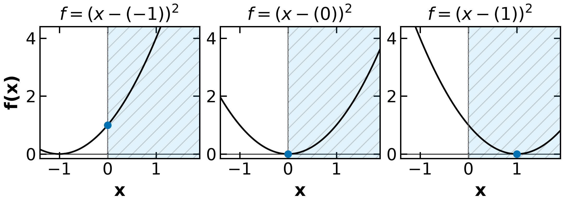
For $\min(x-a)^2$ subject to $-x\le0$, $x^*=\max(a,0)$ and stationarity is $2(x^*-a)-u^*=0$. At $a=-1$, the bound is strongly active with $u^*=2$. At $a=0$, it is weakly active with $u^*=0$. At $a=1$, it is inactive with $u^*=0$. Zero multiplier does not imply slack.

Source: Biegler Def.4.6 and the preceding sets, p.73; the explicit prepared examples supply the distinctions.

Example 4.7: enumerate and test the bound states¶

The Lagrangian and KKT conditions are

Thus $x^*=1/2$, $u_L^*=1$, $u_U^*=0$. The lower bound is strongly active and strict complementarity holds. The objective and bounds are convex, so this candidate is the global minimum. Enumeration considers up to $2^r$ subsets; infeasible or sign-inconsistent branches are rejected, rather than accepted just because some stationarity equations have a root. Active-set and interior-point methods avoid exhaustive enumeration.

Perturb the lower bound to $1/2+\epsilon$. For $-1/2<\epsilon<1/2$, it remains active:

The exact full value function is

For $\epsilon<-1/2$, the lower bound is inactive; at $\epsilon=1/2$ both bounds coincide and the feasible set has one point. Beyond that the problem is infeasible. The original slope 1 predicts only the local linear term; for $\epsilon=0.1$ the true increase is 0.11, not 0.10. Continuing that old line far enough can even predict a negative value for a squared objective.

Weak-activity variation: derive the zero multiplier¶

Now use $\min x^2$ subject to $0\le x\le1$. Write

At $x^*=0$, the upper bound is slack, so complementarity gives $u_U^*=0$. The full stationarity equation then gives $u_L^*=0$. The lower bound is active but weak, and strict complementarity fails. This derives the result without assuming $u_L=0$ in advance. The 2018 scan’s case-ii premise states that value; keeping it in the reference as a source reading does not make it a necessary premise for the derivation.

Perturb the lower bound to $x\ge\epsilon$:

Tightening to $\epsilon>0$ changes the value by $\epsilon^2$; loosening keeps the unconstrained minimizer and changes the value by zero. Both one-sided first derivatives at zero are zero, matching the multiplier. Their second-order behavior differs.

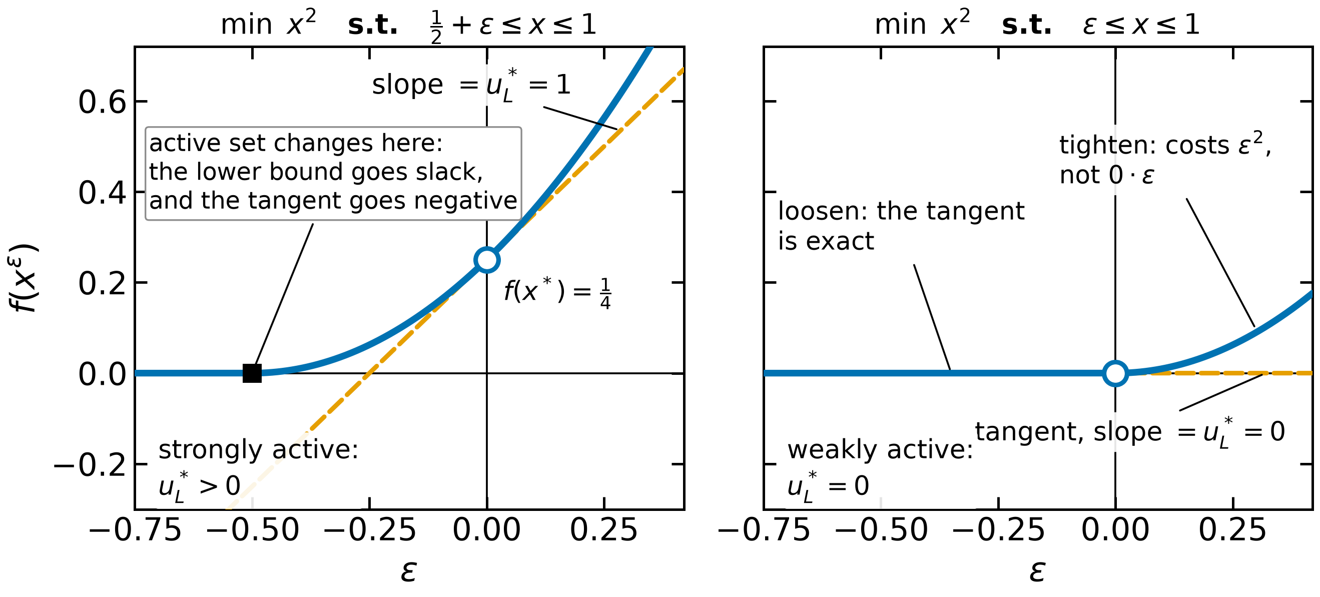
An active-set change requires rechecking the smooth-branch interpretation; it does not automatically destroy the value derivative. Both value functions are continuously differentiable at the slack-to-active transitions shown in the plot ($\epsilon=-1/2$ and $\epsilon=0$), with a change in the second derivative. Their feasibility-domain endpoints are separate: perturbing beyond $1/2$ or 1, respectively, makes the model infeasible. In the weak example the solution branch has different one-sided derivatives, but the value still has derivative zero. For a finite perturbation, recompute the relevant active state and multiplier rather than extrapolating the old slope indefinitely.

Source: Biegler Example 4.7 and variation, pp.73–74. Case enumeration, complete parameter domains and the two-sided qualifications are explicit here.

Computing a branch derivative with the active KKT matrix¶

For twice continuously differentiable data, collect equalities and selected active inequalities into constraint rows $\mathbf J_A$, with multipliers $\boldsymbol\lambda$. A constant right-hand-side perturbation changes one active equation but not its gradient. Differentiating the active stationarity/equality equations of a smooth branch gives

Here $\mathbf e_{\hat\imath}$ is the unit vector in the stacked row corresponding to the perturbed inequality. Its row position includes the equality rows; it is not an unadjusted original inequality index.

This is a derivative of the active KKT equations, not an optimization algorithm. A nonsingular matrix gives one branch derivative. Nocedal & Wright (2006), Appendix A.2, Theorem A.2, p.631, gives the implicit function theorem used here: it supplies a nearby smooth root branch when this active KKT Jacobian is nonsingular; feasibility, multiplier signs and a local sufficiency test are still needed to identify it as the intended minimizer branch. Strictly positive active multipliers and strictly slack inactive constraints persist under small continuous changes; weak activity needs special care.

One sufficient nonsingularity test is full row rank of $\mathbf J_A$ and positive definiteness of $\mathbf W$ on its null space. To verify it, consider a homogeneous solution $(\mathbf p,\mathbf q)$:

Multiplying the first equation by $\mathbf p^T$ gives $\mathbf p^T\mathbf W\mathbf p=0$. Positive curvature on the null space forces $\mathbf p=\mathbf0$. Then $\mathbf J_A^T\mathbf q=\mathbf0$, and full row rank forces $\mathbf q=\mathbf0$. If the active Jacobian is square and nonsingular, its null space is already zero. This explains why the moving-fence/rail toy problem has a well-defined branch even before a nonzero tangent-curvature direction is available.

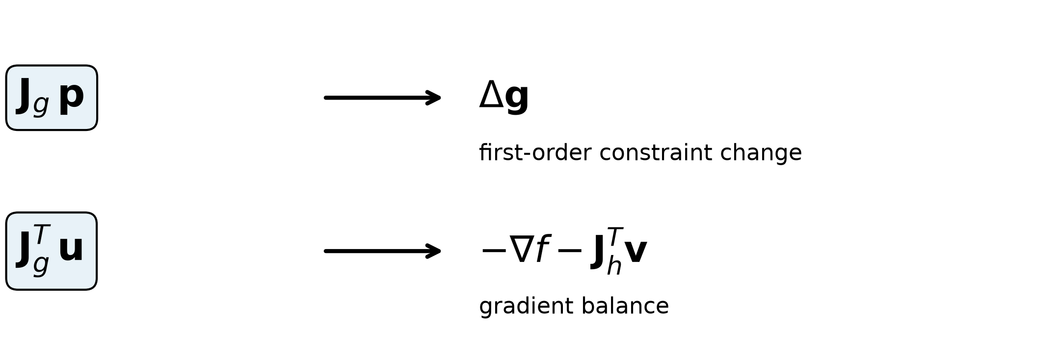
The matrix construction and nonsingularity argument are independently derived from the displayed KKT equations; the extended reduced-Hessian treatment is in Second Order Optimality Conditions.

When the value has two one-sided slopes¶

Consider the convex problem

Its exact value is $V(\epsilon)=\max(\epsilon,0)$. At zero both constraints are active and stationarity is $1-u_1-u_2=0$ with nonnegative multipliers. Every pair $(u_1,u_2)=(t,1-t)$, $0\le t\le1$, is valid. The same primal point therefore has nonunique multipliers. The right value derivative is 1, the left derivative is 0, and there is no ordinary two-sided derivative. The selected constraint multiplier $u_1\in[0,1]$ is a subgradient, not an arbitrary choice of a common slope.

This example also shows why strong/weak labels can depend on the multiplier vector: $(1,0)$ and $(0,1)$ exchange which active constraint is weak. The two gradients are both -1, so LICQ fails, even though a direction $d>0$ strictly decreases both active inequality linearizations.

Rockafellar Thm.9.1 p.224 states a regular-subgradient interpretation under its hypotheses; ordinary partial derivatives follow when the relevant value function is differentiable. Thm.9.3 p.225 gives the convex directional/subgradient relation under its stated existence and lower-semicontinuity hypotheses. In that convex setting, the right and left coordinate slopes are the largest and smallest compatible coordinate multipliers. Those statements should not be read as a global smooth sensitivity theorem for arbitrary nonconvex problems.

The local Taylor proof, the weak squared-value example and this kink example serve different purposes: a smooth branch gives a derivative; a branch switch can leave the value differentiable; nonunique multipliers can describe a range of one-sided sensitivities.

Multipliers in Pyomo¶

Reference: Pyomo Suffix documentation, especially importing solver data and exporting warm-start information. IMPORT retrieves solver-supported suffixes, EXPORT sends them, and IMPORT_EXPORT does both. Names and support depend on the solver/interface. The existing example below uses the Ipopt NL interface: dual for constraint multipliers and ipopt_zL_out/ipopt_zU_out for variable-bound multipliers. The _in suffixes provide the bound-multiplier warm start. Check termination before interpreting any stored suffix, and check the model’s stationarity/sign convention when comparing it with $g\le0$ mathematics.

The warm start below solves the same model again, using the first primal/dual point. It is a demonstration of passing initialization, not a guarantee that warm starting always reduces iterations or selects a global minimum.

Solve without warm starting¶

Inspect dual variables for lower bound

Inspect dual variables for upper bound

Solve with warm starting¶

Translate solver suffixes and check gradient balance¶

For this minimization model and Ipopt NL interface, use the canonical inequality $g=25-x_1x_2x_3x_4\le0$ and equality $h=\sum_i x_i^2-40=0$. The imported inequality dual is $u$, and the equality multiplier in $L=f+u g+v h$ is the negative of the imported equality dual. The canonical lower-bound multiplier is ipopt_zL_out; the canonical upper-bound multiplier is the negative of the signed ipopt_zU_out suffix. Lower-bound multipliers enter stationarity with a minus sign, upper-bound multipliers with a plus sign. Keep the raw signed suffix values when passing a warm start back to the solver. The calculation below checks these signs against independently written analytic gradients, rather than assuming that every solver/interface uses the same suffix convention.

A small residual establishes approximate KKT consistency for this returned point, not a global-minimum certificate for the nonconvex model. The warm-start demonstration repeats the same problem; timing and iteration counts can change with the solver version.

The existing four-variable model has inactive upper bounds. A separate one-variable check, $\min -x$ with $0\le x\le1$, makes the upper bound strongly active and verifies its sign with a nonzero multiplier.