Second Order Optimality Conditions

We test curvature of the Lagrangian, rather than the objective alone. Assume $f$, $g_i$ and $h_j$ are $C^2$ near the point being tested. Use $g_i\le0$, unrestricted equality multipliers, nonnegative inequality multipliers, and row Jacobians. The KKT reference owns the active/strong/weak definitions; the constraint-qualification reference owns feasible paths and tangent versus linearized cones. This page develops the second-order proofs and computational tests used in Lecture 21.

Helpful Cones¶

Linearized and critical directions¶

On open $D\subset\mathbb R^n$, use C$^2$ maps $f:D\to\mathbb R$, $\mathbf g:D\to\mathbb R^r$, $\mathbf h:D\to\mathbb R^m$. At a feasible KKT point $(\mathbf x^*,\mathbf u^*,\mathbf v^*)$, write $\mathcal A_I$ for active inequality indices, split into $\mathcal A_s$ (positive multiplier) and $\mathcal A_w$ (zero multiplier) for the chosen KKT vector. Combined active labels are tagged $(h,j)$ and $(g,i)$; equality 1 and inequality 1 are different constraints. With derivatives evaluated at the point,

At a KKT point, $C_2=C_1\cap\{\nabla f^T\mathbf p=0\}$. Indeed stationarity gives $\nabla f^T\mathbf p=-\sum_{i\in\mathcal A_I}u_i^*\nabla g_i^T\mathbf p\ge0$. Each term is nonnegative; equality to zero forces $\nabla g_i^T\mathbf p=0$ wherever $u_i^*>0$. Weakly active inequalities retain their one-sided restrictions. Biegler (2010), p. 79; Nocedal and Wright (2006), (12.53), p. 330.

Under LICQ, $C_1$ equals the tangent cone, including zero and arbitrary scales. Unit limiting directions are its unit section, as explained in the qualification reference. Neither $C_1$ nor $C_2$ need be a linear subspace.

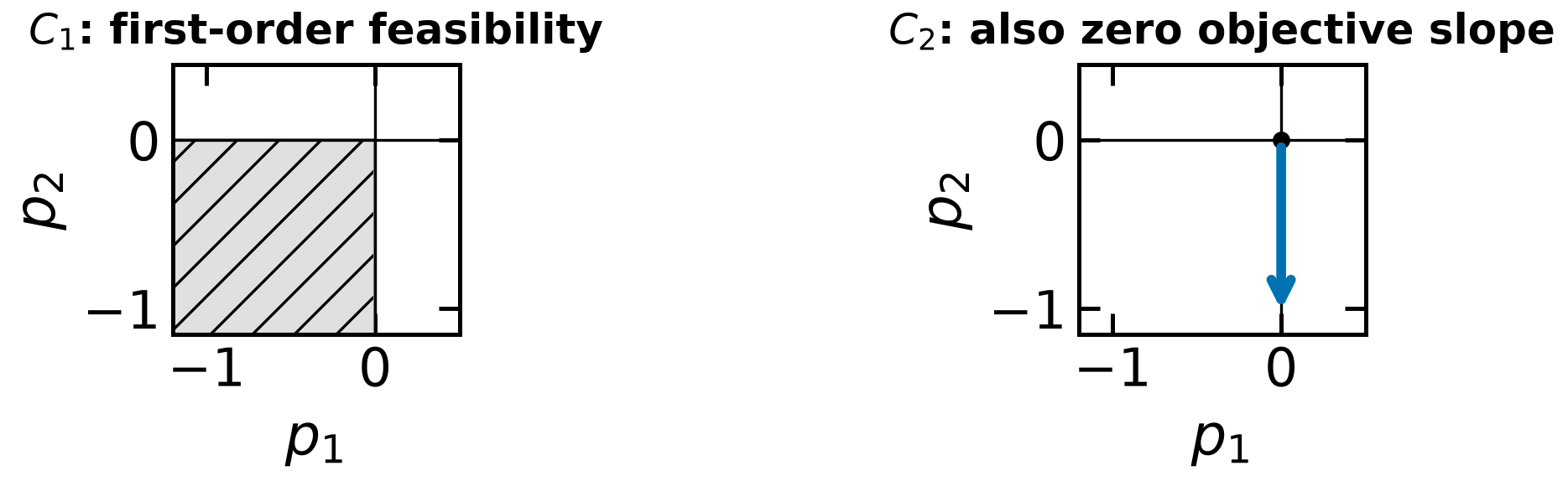
Subspaces that bracket the critical cone¶

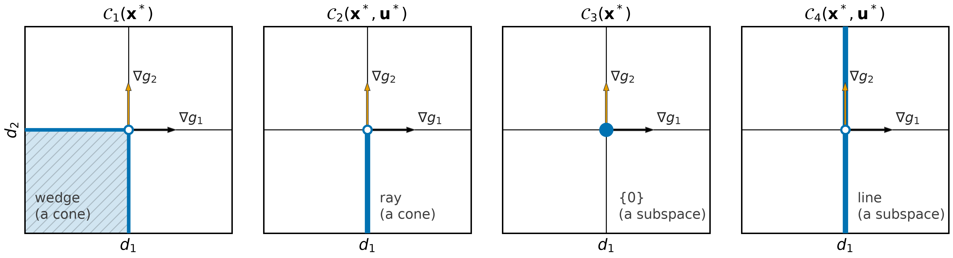
For $g_1=x_1\le0$, $g_2=x_2\le0$, $f=-x_1+x_2^2$, the origin has $(u_1,u_2)=(1,0)$. The panels then show a quadrant ($C_1$), a ray ($C_2$), just zero ($C_3$), and a line ($C_4$). Holding more independent rows at equality makes a smaller subspace.

$C_3$ is contained in $C_4$. Under LICQ the column counts are $n-\operatorname{rows}(\mathbf{A}_3)$ and $n-\operatorname{rows}(\mathbf{A}_4)$; without full row rank use $n-\operatorname{rank}(\mathbf{A}_i)$. A nonempty weak set adds independent rows under LICQ, but strict complementarity makes the two row sets identical. Their null spaces coincide; separately computed bases need not be numerically identical.

Second Order Necessary Conditions¶

Complete necessary-condition proof¶

For $C^2$ data, a local minimum satisfying LICQ has unique KKT multipliers and obeys

This is Biegler’s Theorem 4.17, p. 80 (apply the errata), and Nocedal–Wright’s Theorem 12.5, p. 332.

Complete proof. Fix $\mathbf p\in C_2$. LICQ and the feasible-path construction give $\mathbf z(t)=\mathbf x^*+t\mathbf p+o(t)$ with $h_j(\mathbf z(t))=0$ and each active inequality exactly $g_i(\mathbf z(t))=t\nabla g_i^T\mathbf p\le0$. A strongly active inequality has zero directional derivative; weakly active and inactive constraints have zero multiplier. Thus $L(\mathbf z(t),\mathbf u^*,\mathbf v^*)=f(\mathbf z(t))$ exactly. Stationarity eliminates the linear Taylor term, so

A negative quadratic coefficient dominates the remainder for sufficiently small positive $t$ and contradicts local minimality. This establishes the nonnegative curvature test.

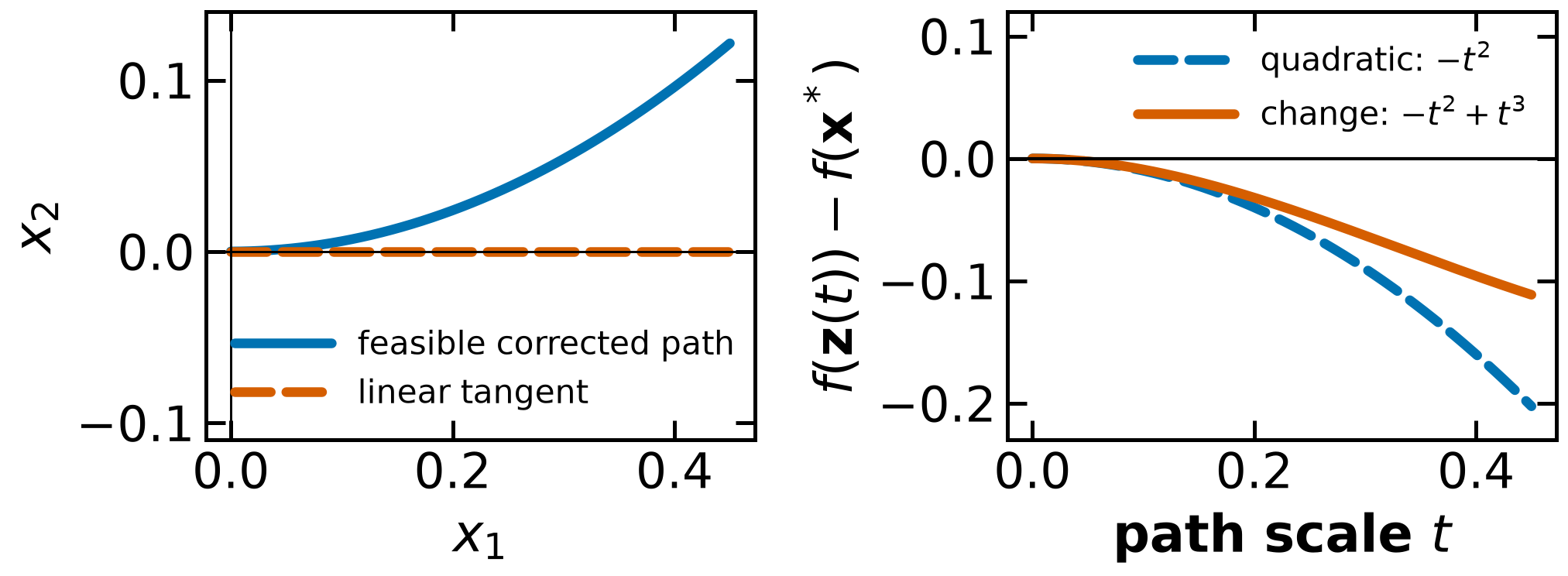
The path correction is $o(t)$; the second-order Taylor remainder is $o(t^2)$. They are different quantities. The vanishing first derivative is what permits the $o(t)$ displacement correction to leave the quadratic coefficient unchanged.

Second Order Sufficient Conditions¶

Complete sufficient-condition proof¶

For $C^2$ data at a KKT point, suppose

Then $\mathbf x^*$ is a strict local minimum. LICQ is not required for this sufficient test. Biegler, Theorem 4.18, pp. 81–82; Nocedal–Wright, Theorem 12.6, pp. 333–334.

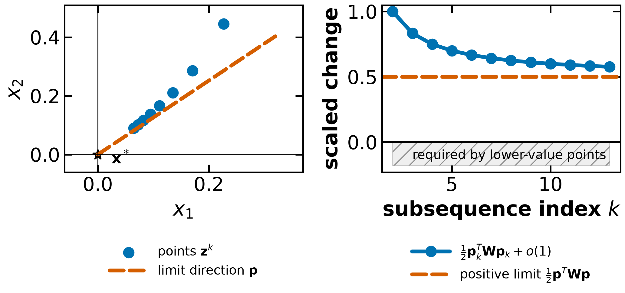
Complete contradiction proof. If strict local minimality fails, choose distinct feasible $\mathbf z^k\to\mathbf x^*$ with $f(\mathbf z^k)\le f(\mathbf x^*)$. Put $r_k=\|\mathbf z^k-\mathbf x^*\|>0$ and $\mathbf p_k=(\mathbf z^k-\mathbf x^*)/r_k$. Compactness of the unit sphere gives a subsequence $\mathbf p_k\to\mathbf p$ with $\|\mathbf p\|=1$. Constraint expansions give $\mathbf p\in C_1$ without any CQ. Dividing the objective difference by $r_k$ gives $\nabla f^T\mathbf p\le0$; stationarity gives $\nabla f^T\mathbf p\ge0$, hence $\mathbf p\in C_2$.

At every feasible point $L(\mathbf z^k,\mathbf u^*,\mathbf v^*)\le f(\mathbf z^k)$ because $\mathbf u^*\ge\mathbf{0}$, $g\le0$ and $h=0$. Also $L(\mathbf x^*,\mathbf u^*,\mathbf v^*)=f(\mathbf x^*)$. The stationary second-order expansion therefore yields

a contradiction. This proof includes directions approaching the critical cone, rather than assuming a direction limit for every original sequence.

Does SOSC imply SONC? At a fixed multiplier vector, strict positivity implies nonnegativity on that same cone. But the necessary-condition theorem additionally assumes LICQ, whereas the sufficient-condition theorem does not. Do not transfer that hypothesis from one theorem to the other. In a degenerate problem different KKT vectors can give different Hessians and critical-cone descriptions; the fixed-vector sufficient test remains meaningful.

In Biegler’s second proof case, all positive-multiplier terms contribute to the first-order Lagrangian/objective difference. Keeping only one chosen negative contribution supports an inequality, not an equality unless the other terms vanish. The argument above keeps the full sum and avoids that omission.

Reduced Hessian¶

A basis for a linear null space¶

For a full-row-rank $\mathbf{A}\in\mathbb R^{m\times n}$ with $m\le n$, a null-space basis $\mathbf{Z}\in\mathbb R^{n\times(n-m)}$ has full column rank and $\mathbf{AZ}=\mathbf{0}$. Every vector in $\ker \mathbf{A}$ is uniquely $\mathbf{Z}\mathbf q$. When $m=n$, the null space is $\{0\}$ and $\mathbf{Z}$ has zero columns; a curvature condition over its nonzero vectors is vacuous.

This is the row-oriented version of Biegler’s Definition 4.19, p. 82. If rows are dependent, the correct dimension is $n-\operatorname{rank}\mathbf{A}$, obtained with a rank-revealing factorization or SVD. Pivoting detects the dependence; it does not make dependent rows independent. An arbitrary critical cone cannot be represented by $\mathbf{Z}\mathbf q$ with unrestricted $\mathbf q$: that image is a subspace.

Complete QR construction and a small worked example¶

For independent rows, factor $\mathbf{A}^T=\mathbf{Q}[\mathbf{R};0]$, where $\mathbf{Q}=[\mathbf{Q}_R\ \mathbf{Q}_N]$ is $n\times n$ orthogonal and $\mathbf{R}$ is nonsingular $m\times m$ upper triangular. Since $\mathbf{Q}_R^T\mathbf{Q}_N=\mathbf{0}$,

and $\mathbf{Q}_N$ has $n-m$ independent columns, so it spans the null space. An economic QR can omit this complement; request the complete factorization. Biegler (4.58), p. 82; Nocedal–Wright (12.74), p. 337.

For $\mathbf{A}=\left[\begin{smallmatrix}1&1&0\\0&1&1\end{smallmatrix}\right]$, choose

Check $\mathbf{A}^T=\mathbf{Q}_R\mathbf{R}$, $\mathbf{AZ}=\mathbf{0}$ and $\mathbf{Z}^T\mathbf{Z}=1$. The two constraint planes intersect in the line spanned by $\mathbf{Z}$.

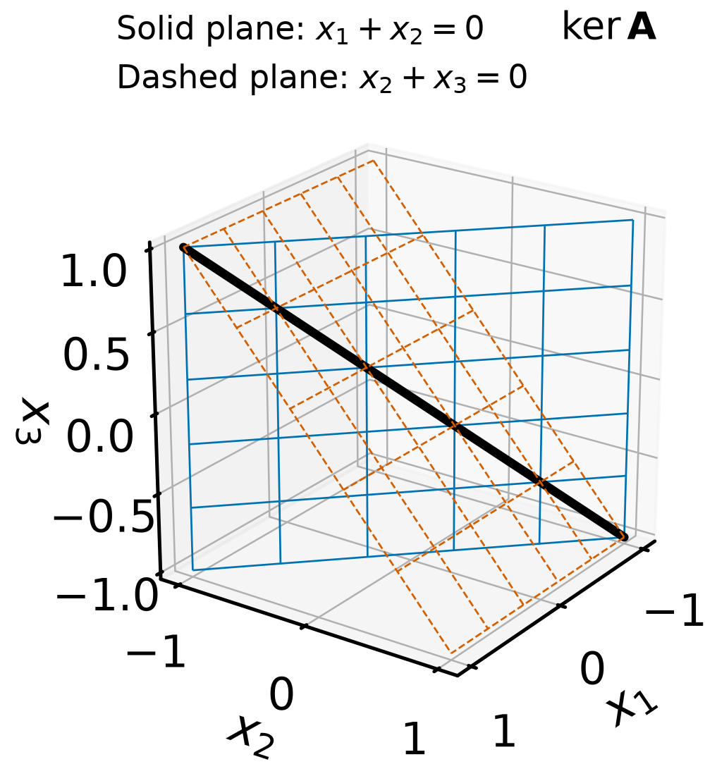
For numerical work use a stable library factorization, inspect the rank threshold, and check $\mathbf{AZ}$, the rank of $\mathbf{Z}$, and $\mathbf{Z}^T\mathbf{Z}$ when an orthonormal basis is intended. Loss of orthogonality does not by itself prove that a full-rank, exactly null basis fails to span the null space. The Math-Primer D3 experiment illustrates orthogonality loss; its economic QR alone does not construct $\mathbf{Q}_N$. Watkins (2002), Sections 3.2–3.3, provides the reflector/rotator background.

Reduced Hessian and basis invariance¶

For symmetric $\mathbf{W}$ and $\mathbf p=\mathbf{Z}\mathbf q$,

Because $\mathbf{Z}$ is a full-rank basis for $\ker \mathbf{A}$, nonzero $\mathbf q$ and nonzero $\mathbf p$ correspond. Thus curvature is positive (semi)definite on this subspace exactly when the reduced Hessian $\mathbf{H}_R=\mathbf{Z}^T\mathbf{WZ}$ is positive (semi)definite. A different basis $\widetilde{\mathbf{Z}}=\mathbf{Z}\mathbf T$, with $T$ nonsingular, gives $\widetilde{\mathbf{H}}_R=\mathbf T^T\mathbf{H}_R\mathbf T$. Definiteness and inertia are invariant; eigenvalue magnitudes generally change. Orthonormal bases make eigenvalue scales easier to interpret.

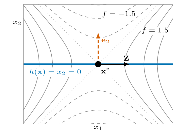
For $f=x_1^2-x_2^2$, $h=x_2=0$, the origin has $v=0$, $\mathbf{W}=\operatorname{diag}(2,-2)$ and $\mathbf{Z}=(1,0)^T$. Its reduced Hessian is 2, so the origin is a strict constrained minimum despite an indefinite full Hessian.

Let $\mathbf{Z}_3,\mathbf{Z}_4$ span $C_3,C_4$. Under the necessary theorem’s hypotheses, $\mathbf{Z}_3^T\mathbf{WZ}_3\succeq0$ is a weaker necessary test because it checks fewer directions. At a KKT point, $\mathbf{Z}_4^T\mathbf{WZ}_4\succ0$ is a stronger sufficient test because it checks more directions than $C_2$ requires. Neither is a general equivalence to the exact cone test.

For example, on $x_1,x_2\ge0$, the function $f=\tfrac12(x_1^2+x_2^2+4x_1x_2)$ has a strict minimum at the origin with zero multipliers. Its critical cone is the nonnegative quadrant. The Hessian $\left[\begin{smallmatrix}1&2\\2&1\end{smallmatrix}\right]$ has eigenvalues 3 and −1, but $\mathbf p^T\mathbf{W}\mathbf p=p_1^2+p_2^2+4p_1p_2>0$ for every nonzero critical direction. The whole-space $C_4$ test fails although the exact SOSC holds. Conversely, the all-active null space can be zero and its necessary test vacuous even at a nonminimum. Strict complementarity makes $C_2=C_3=C_4$, so the subspace tests become exact. Biegler, pp. 82–83.

Example¶

Example 4.20: a positive one-dimensional reduced Hessian¶

Use the canonical positive-domain log model with $g=4-x_1x_2\le0$. Biegler’s Example 4.20 is on p. 83. Its solution is approximately $(1.7981,2.2245)$ with $u=0.5685>0$, so strict complementarity holds. The corrected Lagrangian Hessian is

The gradient row is $\mathbf{J}_g=(-x_2,-x_1)$ and a unit tangent basis is approximately $(-0.6286,0.7777)^T$. The reduced Hessian is about 2.42736 using unrounded values; the errata’s 2.4272 uses the rounded printed basis. The printed 1.0331 and Hessian (4.66) need the errata. With the displayed +9 objective, $f\approx-0.4944$; the book’s −2.4944 is two lower, consistent with +7. The existing source correction explains the constant without changing the derivatives or minimizer.

The Biegler errata corrects p. 83’s Hessian and reduced-Hessian number. The native calculation below preserves the original rounded NumPy example, followed by the actual Pyomo solve and an analytic derivative/basis check. These are numerical evaluations of a supplied model, not a reason to reuse the uncorrected printed matrix.

Calculation with numpy¶

Calculate the complete QR factorization.

The code’s A stacks the single gradient as a column, so A = J_g.T. The second column of the complete $\mathbf{Q}$ lies in $\ker \mathbf{A}^T$, not $\ker \mathbf{A}$. Indeed $\mathbf{A}^T\mathbf{Q}_N=\mathbf{R}^T\mathbf{Q}_R^T\mathbf{Q}_N=\mathbf{0}$. Since $\mathbf{Q}_N$ has the right number of independent columns, it is a basis for the tangent line. Now evaluate $\mathbf{Q}_N^TWQ_N$.

Calculate with Pyomo¶

Define and solve the model¶

Extract the dual variable for the constraint¶

Actual-point derivative and basis check¶

The model and solve above are unchanged. The following cell differentiates the actual Pyomo expressions and archives one shared basis-comparison figure. It records the point before the later experimental barrier calls solve the model again.

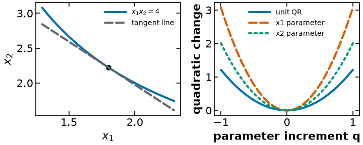
For this canonical upper inequality, the imported Pyomo suffix is negative and $u=-\texttt{m.dual[m.con1]}$ gives the nonnegative canonical multiplier. The analytic stationarity check above verifies the mapping at the actual point. See the KKT suffix reference for other constraint orientations.

The original model comment about changing the inequality to an equality concerns the numerical barrier treatment. At the same point and matching multiplier, the exact active-tangent reduced Hessian is the same; changing a constraint’s role does not by itself change that quadratic form.

Extract the reduced Hessian¶

Compute the reduced Hessian with respect to $x_1$

Compute the reduced Hessian with respect to $x_2$

Coordinate parameters are tangent bases, not coordinate-axis directions¶

At $x_1x_2=4$, the tangent basis for parameter $x_1$ is $Z_{x_1}=(1,-x_2/x_1)^T$, and for parameter $x_2$ it is $Z_{x_2}=(-x_1/x_2,1)^T$. Neither is the coordinate vector $(1,0)^T$ or $(0,1)^T$. Each equals a nonzero scalar multiple of the unit QR basis; consequently its reduced Hessian scales by the square of that scalar. Positive definiteness survives, while the three numerical values differ.

The official experimental API documentation and the installed implementation show that inv_reduced_hessian_barrier solves the model again, forms a barrier-subproblem KKT matrix, and extracts an inverse-Hessian block for selected independent variables. At a finite barrier parameter this is not an exact critical-cone certificate. Its selected variables must be away from their bounds. Check solve status, evaluate the actual active-point derivatives, and distinguish coordinate scaling from finite-barrier and roundoff effects when comparing outputs.