###############################################################################
# The Institute for the Design of Advanced Energy Systems Integrated Platform
# Framework (IDAES IP) was produced under the DOE Institute for the
# Design of Advanced Energy Systems (IDAES).
#
# Copyright (c) 2018-2023 by the software owners: The Regents of the
# University of California, through Lawrence Berkeley National Laboratory,
# National Technology & Engineering Solutions of Sandia, LLC, Carnegie Mellon
# University, West Virginia University Research Corporation, et al.
# All rights reserved.  Please see the files COPYRIGHT.md and LICENSE.md
# for full copyright and license information.
###############################################################################

NLP Diagnostics with Degeneracy Hunter¶

Created by Prof. Alexander Dowling (adowling@nd.edu, University of Notre Dame) and updated by Dr. Andrew Lee (NETL/KeyLogic). The IDAES-PSE examples website and GitHub repository contain the most up-to-date version of this notebook.

Alexander W. Dowling and Lorenz T. Biegler (2015). Degeneracy Hunter: An Algorithm for Determining Irreducible Sets of Degenerate Constraints in Mathematical Programs. 12th International Symposium on Process Systems Engineering and 25th European Symposium on Computer Aided Process Engineering. Ed. by Krist V. Gernaey, Jakob K. Huusom, and Rafiqul Gani. Computer-Aided Chemical Engineering, Vol. 37, p. 809 – 814. link to PDF

Andrew Lee, Robert B. Parker, Sarah Poon, Dan Gunter, Alexander W. Dowling, and Bethany Nicholson (2024). Model Diagnostics for Equation-Oriented Models: Roadblocks and the Path Forward. Foundations of Computer Aided Process Design (FOCAPD 2024), Breckenridge, Colorado, USA, July 14–18, 2024. Peer-reviewed conference proceeding, Systems and Control Transactions, Vol. 3, p. 966 – 974. Lee et al. (2024)

The tools used below are documented in the IDAES reference guide: Diagnostics Toolbox (idaes.core.util.diagnostics_tools.diagnostics_toolbox), SVD Toolbox, and Degeneracy Hunter.

This notebook shows how to use the Degeneracy Hunter tool which is part of the IDAES Diagnostics Toolbox features using two motivating examples:

Inspect constraint violations and bounds of a Pyomo model
Compute the Irreducible Degenerate Set (IDS) for a Pyomo model
Demonstrates the performance benefits in Ipopt from removing a single redundant constraint

Note: Degeneracy Hunter requires a suitable MILP solver. This course example uses `appsi_highs`; SCIP is the default in the toolbox. Select an available MILP solver explicitly.

What does Degeneracy Mean?¶

At a particular point, a selected constraint Jacobian is degenerate when its rows are linearly dependent. A duplicated equation is a simple global example; a nonlinear model can also lose rank only at special states. The simplest example of this is the case where a constraint in the model is duplicated. For example, consider the model below:

\begin{align*} & x_1 + x_2 = 1 \\ & x_1 + x_2 = 1 \\ \end{align*}

(1)

Notice the two equality constraints are identical and thus redundant. This means the constraint qualifications that solvers rely on (e.g., Linear Independence Constraint Qualification or LICQ) do not hold which has three important implications:

Equality multipliers can be nonunique even when the primal minimizer is well defined
The linear systems used by a solver can become singular; bad scaling is a separate issue to check
Theoretical convergence properties of optimization algorithms may not hold

For a square equation-solving problem, counting equations does not establish their independence. These two written equations impose one independent relation, leaving a family of feasible points: any pair of values for x1 and x2 that sums to one. The duplicated equation does not further restrict that family.

In practice, degeneracies are rarely as straight-forward as a duplicated constraint. A more common occurrence is a set of linearly dependent constraints; that is a system of constraints where one constraint in the set can be formed by a linear combination of other constraints in the set. For example:

\begin{align*} & x_1 + x_2 + x_3 = 1 \\ & 2x_1 + 2x_2 + 2x_3 = 2 \\ \end{align*}

(2)

Here, the second constraint can be formed by multiplying the first constraint by two. Another common example of linearly dependent constraints is the combination of a set of material balances for all components in a system and an overall material balance. In this case, the overall material balances can be formed by adding all the individual component balances together. Depending on the number of components being modeled, this system of constraints can be quite large, but the end result is the same; the model effectively has one less constraint than it would appear to have.

The absolute best defense against this is to detect degenerate equations and reformulate the model to remove them; this is the purpose of Degeneracy Hunter. Let’s see it in action.

Setup¶

We start by installing IDAES-PSE, Pyomo, and optimization solvers on Google Colab.

# Imports
import sys

if "google.colab" in sys.modules:
    !wget "https://raw.githubusercontent.com/ndcbe/optimization/main/notebooks/helper.py"
    import helper

    helper.easy_install()
else:
    sys.path.insert(0, "../")
    import helper
helper.set_plotting_style()

Next, we import Pyomo and the IDAES Diagnostics Toolbox.

import pyomo.environ as pyo

from idaes.core.util.diagnostics_tools.diagnostics_toolbox import DiagnosticsToolbox

from idaes.core.util.testing import _enable_scip_solver_for_testing

"""
scip_solver = pyo.SolverFactory("scip")
if not scip_solver.available():
    _enable_scip_solver_for_testing()
assert scip_solver.available()
"""
print(" ")
# We currently do not install scip on Colab

Example: Linear Program with Redundant Equality Constraints¶

Let’s apply these tools to a poorly formulated optimization problem:

\begin{align*} \min_{\mathbf{x}} \quad & \sum_{i=\{1,...,3\}} x_i \\ \mathrm{s.t.}~~& x_1 + x_2 \geq 1 \\ & x_1 + x_2 + x_3 = 1 \\ & x_2 - 2 x_3 \leq 1 \\ & x_1 + x_3 \geq 1 \\ & x_1 + x_2 + x_3 = 1 \\ \end{align*}

(3)

As you can see, this is similar to our example above with duplicated equality constraints.

The cell below shows how to construct this model in Pyomo.

def build_example(include_redundant_constraint=True):
    """Build the test model with an optional duplicate equality."""
    m = pyo.ConcreteModel()

    m.I = pyo.Set(initialize=[i for i in range(1, 4)])

    m.x = pyo.Var(m.I, bounds=(0, 5), initialize=1.0)

    m.con1 = pyo.Constraint(expr=m.x[1] + m.x[2] >= 1)
    m.con2 = pyo.Constraint(expr=m.x[1] + m.x[2] + m.x[3] == 1)
    m.con3 = pyo.Constraint(expr=m.x[2] - 2 * m.x[3] <= 1)
    m.con4 = pyo.Constraint(expr=m.x[1] + m.x[3] >= 1)

    if include_redundant_constraint:
        m.con5 = pyo.Constraint(expr=m.x[1] + m.x[2] + m.x[3] == 1)

    m.obj = pyo.Objective(expr=sum(m.x[i] for i in m.I))

    return m


m = build_example()

Check for Structural Issues¶

Before we try to solve the model, the first thing we should do is use the Diagnostics Toolbox to check for any structural issues in our model. The cell below creates an instance of the Diagnostics Toolbox and calls the report_structural_issues method.

dt = DiagnosticsToolbox(m)
dt.report_structural_issues()

====================================================================================
Model Statistics

        Activated Blocks: 1 (Deactivated: 0)
        Free Variables in Activated Constraints: 3 (External: 0)
            Free Variables with only lower bounds: 0
            Free Variables with only upper bounds: 0
            Free Variables with upper and lower bounds: 3
        Fixed Variables in Activated Constraints: 0 (External: 0)
        Activated Equality Constraints: 2 (Deactivated: 0)
        Activated Inequality Constraints: 3 (Deactivated: 0)
        Activated Objectives: 1 (Deactivated: 0)

------------------------------------------------------------------------------------
2 WARNINGS

    WARNING: 1 Degree of Freedom
    WARNING: Structural singularity found
        Under-Constrained Set: 3 variables, 2 constraints
        Over-Constrained Set: 0 variables, 0 constraints

------------------------------------------------------------------------------------
0 Cautions

    No cautions found!

------------------------------------------------------------------------------------
Suggested next steps:

    display_underconstrained_set()

====================================================================================

The toolbox reports one degree of freedom by counting three free variables and two written equalities. Those equalities are duplicates: their numerical Jacobian has only one independent row, leaving two equality-feasible directions before inequalities and bounds are considered. The structural under-constrained pattern is compatible with free optimization variables, but the equation count alone does not establish independence. Keep the duplicate in this intentional experiment and inspect numerical rank below.

solver = pyo.SolverFactory("ipopt")

# Specifying an iteration limit of 0 allows us to inspect the initial point
solver.options["max_iter"] = 0

# "Solving" the model with an iteration limit of 0 load the initial point and applies
# any preprocessors (e.g., enforces bounds)
results = solver.solve(m, tee=True)

# max_iter = 0 means Ipopt is EXPECTED to stop on the iteration limit here.
# Check for that rather than for optimality (Pyomo style guide, section 7).
assert (
    results.solver.termination_condition == pyo.TerminationCondition.maxIterations
), f"expected to stop at the iteration limit, got {results.solver.termination_condition}"

Ipopt 3.13.2: max_iter=0


******************************************************************************
This program contains Ipopt, a library for large-scale nonlinear optimization.
 Ipopt is released as open source code under the Eclipse Public License (EPL).
         For more information visit http://projects.coin-or.org/Ipopt

This version of Ipopt was compiled from source code available at
    https://github.com/IDAES/Ipopt as part of the Institute for the Design of
    Advanced Energy Systems Process Systems Engineering Framework (IDAES PSE
    Framework) Copyright (c) 2018-2019. See https://github.com/IDAES/idaes-pse.

This version of Ipopt was compiled using HSL, a collection of Fortran codes
    for large-scale scientific computation.  All technical papers, sales and
    publicity material resulting from use of the HSL codes within IPOPT must
    contain the following acknowledgement:
        HSL, a collection of Fortran codes for large-scale scientific
        computation. See http://www.hsl.rl.ac.uk.
******************************************************************************

This is Ipopt version 3.13.2, running with linear solver ma27.

Number of nonzeros in equality constraint Jacobian...:        6
Number of nonzeros in inequality constraint Jacobian.:        6
Number of nonzeros in Lagrangian Hessian.............:        0

Total number of variables............................:        3
                     variables with only lower bounds:        0
                variables with lower and upper bounds:        3
                     variables with only upper bounds:        0
Total number of equality constraints.................:        2
Total number of inequality constraints...............:        3
        inequality constraints with only lower bounds:        2
   inequality constraints with lower and upper bounds:        0
        inequality constraints with only upper bounds:        1

iter    objective    inf_pr   inf_du lg(mu)  ||d||  lg(rg) alpha_du alpha_pr  ls
   0  3.0000000e+00 2.00e+00 1.00e+00  -1.0 0.00e+00    -  0.00e+00 0.00e+00   0

Number of Iterations....: 0

                                   (scaled)                 (unscaled)
Objective...............:   3.0000000000000000e+00    3.0000000000000000e+00
Dual infeasibility......:   1.0000000000000000e+00    1.0000000000000000e+00
Constraint violation....:   2.0000000000000000e+00    2.0000000000000000e+00
Complementarity.........:   4.0000000499999997e+00    4.0000000499999997e+00
Overall NLP error.......:   4.0000000499999997e+00    4.0000000499999997e+00


Number of objective function evaluations             = 1
Number of objective gradient evaluations             = 1
Number of equality constraint evaluations            = 1
Number of inequality constraint evaluations          = 1
Number of equality constraint Jacobian evaluations   = 1
Number of inequality constraint Jacobian evaluations = 1
Number of Lagrangian Hessian evaluations             = 0
Total CPU secs in IPOPT (w/o function evaluations)   =      0.000
Total CPU secs in NLP function evaluations           =      0.000

EXIT: Maximum Number of Iterations Exceeded.

WARNING: Loading a SolverResults object with a warning status into
model.name="unknown";
    - termination condition: maxIterations
    - message from solver: Ipopt 3.13.2\x3a Maximum Number of Iterations
      Exceeded.

Identify constraints with large residuals at the initial point¶

With the solution at the initial point, we can then use the Diagnostics Toolbox to check the residuals of all constraints at the initial point.

# Check for large residuals
dt.display_constraints_with_large_residuals()

====================================================================================
The following constraint(s) have large residuals (>1.0E-05):

    con2: 2.00000E+00
    con5: 2.00000E+00

====================================================================================

We can also check for variables which are close to (or outside of) their bounds.

dt.display_variables_near_bounds()

====================================================================================
The following variable(s) have values close to their bounds (abs=1.0E-04, rel=1.0E-04):


====================================================================================

The initial point has residuals to correct, and the duplicate equality remains. Proceed with this intentionally degenerate model to observe how the solver handles it.

solver.options["max_iter"] = 50
results = solver.solve(m, tee=True)
assert pyo.check_optimal_termination(results), (
    f"Solve failed: status={results.solver.status}, "
    f"termination={results.solver.termination_condition}"
)

Ipopt 3.13.2: max_iter=50


******************************************************************************
This program contains Ipopt, a library for large-scale nonlinear optimization.
 Ipopt is released as open source code under the Eclipse Public License (EPL).
         For more information visit http://projects.coin-or.org/Ipopt

This version of Ipopt was compiled from source code available at
    https://github.com/IDAES/Ipopt as part of the Institute for the Design of
    Advanced Energy Systems Process Systems Engineering Framework (IDAES PSE
    Framework) Copyright (c) 2018-2019. See https://github.com/IDAES/idaes-pse.

This version of Ipopt was compiled using HSL, a collection of Fortran codes
    for large-scale scientific computation.  All technical papers, sales and
    publicity material resulting from use of the HSL codes within IPOPT must
    contain the following acknowledgement:
        HSL, a collection of Fortran codes for large-scale scientific
        computation. See http://www.hsl.rl.ac.uk.
******************************************************************************

This is Ipopt version 3.13.2, running with linear solver ma27.

Number of nonzeros in equality constraint Jacobian...:        6
Number of nonzeros in inequality constraint Jacobian.:        6
Number of nonzeros in Lagrangian Hessian.............:        0

Total number of variables............................:        3
                     variables with only lower bounds:        0
                variables with lower and upper bounds:        3
                     variables with only upper bounds:        0
Total number of equality constraints.................:        2
Total number of inequality constraints...............:        3
        inequality constraints with only lower bounds:        2
   inequality constraints with lower and upper bounds:        0
        inequality constraints with only upper bounds:        1

iter    objective    inf_pr   inf_du lg(mu)  ||d||  lg(rg) alpha_du alpha_pr  ls
   0  3.0000000e+00 2.00e+00 1.00e+00  -1.0 0.00e+00    -  0.00e+00 0.00e+00   0
   1  1.3934810e+00 3.93e-01 2.17e-01  -1.0 1.23e+00    -  7.90e-01 8.03e-01h  1
   2  1.0184419e+00 1.84e-02 1.26e-02  -1.7 7.02e-01    -  9.41e-01 9.53e-01h  1
   3  1.0011246e+00 1.12e-03 3.82e-02  -2.5 1.50e-02    -  1.00e+00 9.39e-01h  1
   4  1.0006914e+00 6.91e-04 3.12e+00  -2.5 3.17e-03    -  1.00e+00 3.85e-01h  1
   5  1.0002664e+00 2.66e-04 4.35e+00  -2.5 1.12e-03    -  1.00e+00 6.15e-01h  1
   6  1.0001115e+00 1.12e-04 1.07e+01  -2.5 4.99e-04    -  1.00e+00 5.82e-01h  1
   7  1.0000788e+00 7.88e-05 4.33e+01  -2.5 1.88e-04    -  1.00e+00 2.94e-01f  2
   8  1.0000153e+00 1.53e-05 2.19e+01  -2.5 6.85e-05    -  1.00e+00 8.08e-01h  1
   9  1.0000118e+00 1.18e-05 2.78e+02  -2.5 3.47e-05    -  1.00e+00 2.45e-01f  2
iter    objective    inf_pr   inf_du lg(mu)  ||d||  lg(rg) alpha_du alpha_pr  ls
  10  1.0000014e+00 1.44e-06 2.83e-08  -2.5 7.79e-06    -  1.00e+00 1.00e+00h  1
  11  1.0000000e+00 1.39e-09 1.84e-11  -5.7 2.56e-06    -  1.00e+00 1.00e+00h  1
  12  1.0000000e+00 1.39e-09 1.24e+02  -8.6 1.16e-08    -  1.00e+00 9.54e-07h 21
  13  9.9999999e-01 9.82e-09 1.84e-13  -8.6 1.33e-08    -  1.00e+00 1.00e+00s 22
  14  9.9999999e-01 9.96e-09 1.63e-13  -8.6 2.29e-10    -  1.00e+00 1.00e+00s 22
  15  9.9999999e-01 9.96e-09 1.82e+02  -9.0 4.00e-11    -  1.00e+00 9.54e-07h 21
  16  9.9999999e-01 1.00e-08 1.94e-13  -9.0 5.89e-11    -  1.00e+00 1.00e+00s 22

Number of Iterations....: 16

                                   (scaled)                 (unscaled)
Objective...............:   9.9999999000238915e-01    9.9999999000238915e-01
Dual infeasibility......:   1.9444755585626268e-13    1.9444755585626268e-13
Constraint violation....:   9.9976108502985994e-09    9.9976108502985994e-09
Complementarity.........:   9.2217032157601162e-10    9.2217032157601162e-10
Overall NLP error.......:   9.9976108502985994e-09    9.9976108502985994e-09


Number of objective function evaluations             = 111
Number of objective gradient evaluations             = 17
Number of equality constraint evaluations            = 111
Number of inequality constraint evaluations          = 111
Number of equality constraint Jacobian evaluations   = 17
Number of inequality constraint Jacobian evaluations = 17
Number of Lagrangian Hessian evaluations             = 16
Total CPU secs in IPOPT (w/o function evaluations)   =      0.002
Total CPU secs in NLP function evaluations           =      0.000

EXIT: Optimal Solution Found.

Ipopt reaches a reported optimum despite the duplicated equality. Inspect both ls (line-search trial count) and alpha_pr (accepted primal step fraction). One trial does not mean a full step: several early rows have alpha_pr < 1. Iterations 12–16 use 21 or 22 trials, indicating extra work near the solution. The deliberate failure mode is the redundant equation, not a coding error to remove before diagnosis.

The cell below shows the variable values.

m.x.display()

x : Size=3, Index=I
    Key : Lower : Value              : Upper : Fixed : Stale : Domain
      1 :     0 : 1.0000000099975996 :     5 : False : False :  Reals
      2 :     0 :                0.0 :     5 : False : False :  Reals
      3 :     0 :                0.0 :     5 : False : False :  Reals

Check the rank of the Jacobian of the equality constraints¶

One way to check for the presence of degenerate equations is to calculate the rank of the Jacobian matrix of the equality constraints. Small singular values identify numerical rank at a chosen tolerance; inspect scaling before calling them exact dependencies. In this example the duplicated rows independently establish an exact dependence.

The Diagnostics Toolbox contains a Singular Value Decomposition (SVD) toolbox which can be used to determine the number of small singular values in the Jacobian for a model as shown below.

svd = dt.prepare_svd_toolbox()
svd.display_rank_of_equality_constraints()

====================================================================================

Number of Singular Values less than 1.0E-06 is 1

====================================================================================

As can be seen above, there is one singular value less than 1e-6, suggesting we have one degenerate constraint.

Finding Irreducible Degenerate Sets (IDS)¶

Next, we can use Degeneracy Hunter to identify irreducible degenerate sets; that is, a dependent set of constraint rows with no proper dependent subset.

Degeneracy Hunter first identifies candidate degenerate equations by solving a mixed integer linear program (MILP). It then iterates through the candidate equations and solves a second MILP for each to compute the irreducible degenerate set that must contain the candidate equation.

Note: Degeneracy Hunter requires a suitable MILP solver, users can specify their solver of choice via a configuration argument. The default option is SCIP (https://scipopt.org/) which is an open-source solver.

The cell below shows how to create an instance of Degeneracy Hunter and generate a report of the irreducible degenerate sets.

# dh = dt.prepare_degeneracy_hunter() # default solver is scip
dh = dt.prepare_degeneracy_hunter(solver="appsi_highs")
dh.report_irreducible_degenerate_sets()

2026-10-13 16:27:49 [INFO] idaes.core.util.diagnostics_tools.degeneracy_hunter: Searching for Candidate Equations

2026-10-13 16:27:49 [INFO] idaes.core.util.diagnostics_tools.degeneracy_hunter: Building MILP model.

2026-10-13 16:27:49 [INFO] idaes.core.util.diagnostics_tools.degeneracy_hunter: Solving Candidates MILP model.

2026-10-13 16:27:49 [INFO] idaes.core.util.diagnostics_tools.degeneracy_hunter: Searching for Irreducible Degenerate Sets

2026-10-13 16:27:49 [INFO] idaes.core.util.diagnostics_tools.degeneracy_hunter: Building MILP model to compute irreducible degenerate set.

Solving MILP 1 of 2.
2026-10-13 16:27:49 [INFO] idaes.core.util.diagnostics_tools.degeneracy_hunter: Solving IDS MILP for constraint con2.

Solving MILP 2 of 2.
2026-10-13 16:27:49 [INFO] idaes.core.util.diagnostics_tools.degeneracy_hunter: Solving IDS MILP for constraint con5.

====================================================================================
Irreducible Degenerate Sets

    Irreducible Degenerate Set 0
        nu    Constraint Name
        1.0   con2
        -1.0  con5

    Irreducible Degenerate Set 1
        nu    Constraint Name
        -1.0  con2
        1.0   con5

====================================================================================

As can be seen above, Degeneracy Hunter identified two constraints as potentially redundant (the duplicate constraints con2 and con5). Degeneracy Hunter then reports an Irreducible Degenerate Set for each of these constraints, which in the case as identical. More complex models may have partially overlapping IDS’s.

These results show us that con2 and con5 are mutually redundant; i.e., we can eliminate one of these with no effect on the model solution.

Reformulate Model to Remove Redundant Constraint¶

Now let’s reformulate the model by removing the redundant equality constraint con5 and solve the reformulated model.

m2 = build_example(include_redundant_constraint=False)

results = solver.solve(m2, tee=True)
assert pyo.check_optimal_termination(results), (
    f"Solve failed: status={results.solver.status}, "
    f"termination={results.solver.termination_condition}"
)

Ipopt 3.13.2: max_iter=50


******************************************************************************
This program contains Ipopt, a library for large-scale nonlinear optimization.
 Ipopt is released as open source code under the Eclipse Public License (EPL).
         For more information visit http://projects.coin-or.org/Ipopt

This version of Ipopt was compiled from source code available at
    https://github.com/IDAES/Ipopt as part of the Institute for the Design of
    Advanced Energy Systems Process Systems Engineering Framework (IDAES PSE
    Framework) Copyright (c) 2018-2019. See https://github.com/IDAES/idaes-pse.

This version of Ipopt was compiled using HSL, a collection of Fortran codes
    for large-scale scientific computation.  All technical papers, sales and
    publicity material resulting from use of the HSL codes within IPOPT must
    contain the following acknowledgement:
        HSL, a collection of Fortran codes for large-scale scientific
        computation. See http://www.hsl.rl.ac.uk.
******************************************************************************

This is Ipopt version 3.13.2, running with linear solver ma27.

Number of nonzeros in equality constraint Jacobian...:        3
Number of nonzeros in inequality constraint Jacobian.:        6
Number of nonzeros in Lagrangian Hessian.............:        0

Total number of variables............................:        3
                     variables with only lower bounds:        0
                variables with lower and upper bounds:        3
                     variables with only upper bounds:        0
Total number of equality constraints.................:        1
Total number of inequality constraints...............:        3
        inequality constraints with only lower bounds:        2
   inequality constraints with lower and upper bounds:        0
        inequality constraints with only upper bounds:        1

iter    objective    inf_pr   inf_du lg(mu)  ||d||  lg(rg) alpha_du alpha_pr  ls
   0  3.0000000e+00 2.00e+00 6.30e-01  -1.0 0.00e+00    -  0.00e+00 0.00e+00   0
   1  1.3934810e+00 3.93e-01 1.34e-01  -1.0 1.23e+00    -  7.90e-01 8.03e-01f  1
   2  1.0184419e+00 1.84e-02 9.15e-03  -1.7 7.02e-01    -  9.41e-01 9.53e-01h  1
   3  1.0011246e+00 1.12e-03 3.88e-02  -2.5 1.50e-02    -  1.00e+00 9.39e-01h  1
   4  1.0006914e+00 6.91e-04 3.12e+00  -2.5 3.17e-03    -  1.00e+00 3.85e-01h  1
   5  1.0002664e+00 2.66e-04 4.35e+00  -2.5 1.12e-03    -  1.00e+00 6.15e-01h  1
   6  1.0001115e+00 1.12e-04 1.07e+01  -2.5 5.00e-04    -  1.00e+00 5.81e-01h  1
   7  1.0000788e+00 7.88e-05 4.34e+01  -2.5 1.88e-04    -  1.00e+00 2.93e-01f  2
   8  1.0000154e+00 1.54e-05 2.26e+01  -2.5 6.89e-05    -  1.00e+00 8.04e-01h  1
   9  1.0000118e+00 1.18e-05 2.98e+02  -2.5 3.64e-05    -  1.00e+00 2.33e-01f  2
iter    objective    inf_pr   inf_du lg(mu)  ||d||  lg(rg) alpha_du alpha_pr  ls
  10  1.0000020e+00 2.04e-06 1.33e+02  -2.5 9.72e-06    -  1.00e+00 8.28e-01h  1
  11  1.0000016e+00 1.61e-06 2.26e+03  -2.5 4.79e-06    -  1.00e+00 2.12e-01f  2
  12  1.0000002e+00 2.46e-07 8.72e+02  -2.5 1.20e-06    -  1.00e+00 8.47e-01h  1
  13  1.0000002e+00 1.95e-07 1.71e+04  -2.5 7.02e-07    -  1.00e+00 2.09e-01f  2
  14  1.0000000e+00 1.54e-08 3.23e+03  -2.5 1.50e-07    -  1.00e+00 9.21e-01h  1
  15  1.0000000e+00 1.15e-08 9.99e+04  -2.5 6.89e-08    -  1.00e+00 2.54e-01f  2
  16  1.0000000e+00 2.22e-16 2.83e-08  -2.5 8.21e-09    -  1.00e+00 1.00e+00h  1
  17  1.0000000e+00 1.11e-16 2.86e-11  -8.6 8.25e-16    -  1.00e+00 1.00e+00   0

Number of Iterations....: 17

                                   (scaled)                 (unscaled)
Objective...............:   9.9999999999999989e-01    9.9999999999999989e-01
Dual infeasibility......:   2.8586412100309322e-11    2.8586412100309322e-11
Constraint violation....:   1.1102230246251565e-16    1.1102230246251565e-16
Complementarity.........:   2.6658012064298784e-09    2.6658012064298784e-09
Overall NLP error.......:   2.6658012064298784e-09    2.6658012064298784e-09


Number of objective function evaluations             = 23
Number of objective gradient evaluations             = 18
Number of equality constraint evaluations            = 23
Number of inequality constraint evaluations          = 23
Number of equality constraint Jacobian evaluations   = 18
Number of inequality constraint Jacobian evaluations = 18
Number of Lagrangian Hessian evaluations             = 17
Total CPU secs in IPOPT (w/o function evaluations)   =      0.001
Total CPU secs in NLP function evaluations           =      0.000

EXIT: Optimal Solution Found.

First, let us check to see if the optimal solution has changed.

m2.x.display()

x : Size=3, Index=I
    Key : Lower : Value                  : Upper : Fixed : Stale : Domain
      1 :     0 :     1.0000000005924994 :     5 : False : False :  Reals
      2 :     0 :                    0.0 :     5 : False : False :  Reals
      3 :     0 : 4.5584432539719464e-11 :     5 : False : False :  Reals

We get the same answer as before, but careful inspection of the Ipopt output reveals a subtle improvement. Notice ls is only 1 or 2 for all of the iterations, in contrast to more than 20 for the original model. The accepted step fractions still vary; fewer trials do not mean that every step is full.

Let’s also compare the number of function evaluations.

Original model (using Ipopt 3.13.2 with ma27):

Number of objective function evaluations             = 111
Number of objective gradient evaluations             = 17
Number of equality constraint evaluations            = 111
Number of inequality constraint evaluations          = 111
Number of equality constraint Jacobian evaluations   = 17
Number of inequality constraint Jacobian evaluations = 17
Number of Lagrangian Hessian evaluations             = 16

Reformulated model (using Ipopt 3.13.2 with ma27):

Number of objective function evaluations             = 23
Number of objective gradient evaluations             = 18
Number of equality constraint evaluations            = 23
Number of inequality constraint evaluations          = 23
Number of equality constraint Jacobian evaluations   = 18
Number of inequality constraint Jacobian evaluations = 18
Number of Lagrangian Hessian evaluations             = 17

Removing a single redundant constraint reduced the number of objective and constraint evaluations from 111 to 23, about 4.83 times fewer in this run. The iteration count increases from 16 to 17; the benefit is fewer function evaluations, not fewer iterations.

Often degenerate equations have a much worse impact on large-scale problems; for example, degenerate equations can cause Ipopt to require many more iterations or terminate at an infeasible point.

import pytest

# This ensures the model answer is correct.
# This is helpful for testing the notebook.
# As a student, you can ignore this. You do not need it.
assert pyo.value(m2.x[1]) == pytest.approx(1, rel=1e-6)
assert pyo.value(m2.x[2]) == pytest.approx(0, abs=1e-6)
assert pyo.value(m2.x[3]) == pytest.approx(0, abs=1e-6)

Reference: what a degeneracy diagnostic establishes¶

For the canonical NLP, LICQ tests all equality rows and all active inequality rows, including weakly active inequalities and active bounds. A diagnostic restricted to equalities, or to equalities and strongly active inequalities, establishes dependence for that selected matrix; independence of a subset does not prove full LICQ. The 2015 algorithm admits weakly active rows as an option. Record the point, scaling, activity tolerance, multiplier tolerance, and selected rows with a report.

For a selected row matrix $\mathbf A\in\mathbb R^{n_a\times n}$ , degeneracy means $\operatorname{rank}\mathbf A<n_a$ . An irreducible row index set $I$ is dependent and every proper subset $J\subsetneq I$ is independent.

A selected Jacobian is globally degenerate when its rows are dependent throughout the relevant model domain, and locally degenerate when rank is lost at a particular state. Duplicated balances and equations implied by other equations are global examples. Local degeneracy can occur when a unit disappears: in $F=V+L$ , $Fz_i=Lx_i+Vy_i$ , derivatives of the component residual with respect to $z_i,x_i,y_i$ vanish at zero flows. This observation alone does not prove rank loss of the entire model; inspect the remaining equations and columns. Degeneracy can also describe a valid model at a special state or a legitimate constrained corner. It is a hypothesis failure to diagnose, not automatic proof of a modeling mistake.

If each component balance is $r_i=Fz_i-Lx_i-Vy_i=0$ , then $\sum_i r_i=F-L-V$ on the normalized-composition manifold $\sum_i z_i=\sum_i x_i=\sum_i y_i=1$ . Adding the overall balance together with the component balances and composition-normalization equations creates a row dependence. If the normalizations are variable equations, include their gradients in the dependence: do not assert $\nabla r_{\mathrm{overall}}=\sum_i\nabla r_i$ in unrestricted composition coordinates.

For any equality-row dependence $\mathbf J_h^T\boldsymbol\nu=0$ , $\boldsymbol\nu\ne0$ , the equality KKT matrix has null vector

\begin{bmatrix}\mathbf W&\mathbf J_h^T\\\mathbf J_h&\mathbf0\end{bmatrix}\begin{bmatrix}\mathbf0\\\boldsymbol\nu\end{bmatrix}=\mathbf0.

(4)

Its linear step cannot have a unique solution; it may also be inconsistent. At a KKT point, unrestricted equality multipliers move as $\mathbf v+t\boldsymbol\nu$ . Individual redundant-equation prices are not identifiable; invariant combinations can still carry information. For dependent inequality rows, sign restrictions can leave a unique multiplier, so the equality conclusion must not be generalized without checking signs. See the constraint-qualification reference.

Historically, active-set solvers can omit dependent rows from a working system and interior-point solvers regularize their linear systems. These safeguards do not repair the model, and modern implementations have additional strategies. Do not blindly delete an equation from a zero-flow local degeneracy: doing so can discard a conservation law away from that state. Dowling and Biegler (2015), Degeneracy Hunter: An Algorithm for Determining Irreducible Sets of Degenerate Constraints in Mathematical Programs, pp. 809–811, DOI.

Irreducible sets and the candidate MILP¶

An irreducible degenerate set is a dependent set of rows with no proper dependent subset (inclusion minimal). Different irreducible sets may have different sizes. A minimum-cardinality dependence is irreducible, but an arbitrary irreducible set need not be the smallest one in the whole matrix.

The original four-step workflow is: (1) select/scale Jacobian rows using the iterate and activity information; (2) QR-factorize and identify nonpivot candidate rows; (3) solve a sparse-dependence MILP for each candidate; (4) report constraint names and dependence coefficients. With selected row matrix $\mathbf A$ , candidate $j$ , and a sufficiently large finite $M$ :

\begin{aligned}\min_{\boldsymbol\lambda,\mathbf y}\quad&\sum_i y_i\\ \text{s.t.}\quad&\mathbf A^T\boldsymbol\lambda=\mathbf0,\\ &-My_i\le\lambda_i\le My_i,\\ &\lambda_j=1,\quad\mathbf y\in\{0,1\}^{n_a}.\end{aligned}

(5)

$\mathbf A^T\boldsymbol\lambda=\mathbf0$ detects a row dependence; binary $y_i$ counts its support; fixing $\lambda_j=1$ excludes the trivial solution and requires the candidate’s participation. An optimal MILP finds a minimum-cardinality admissible dependence containing that candidate. Cycling candidates can expose several sets, and tied solutions may need enumeration. It is not a guarantee that one solve returns every irreducible set. Finite $M$ and tolerances can exclude a normalized dependence; MILP infeasibility may reflect that limitation or numerical QR noise, so inspect scaling, coefficients, termination and tolerances before declaring no dependence. Dowling and Biegler, Algorithm 1 and (4), pp. 811–812.

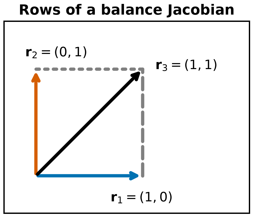
Rows that form a three-equation dependence

For rows $(1,0),(0,1),(1,1)$ , the dependence is $r_1+r_2-r_3=0$ . Every pair is independent, so all three rows form an irreducible set. This is a small algebraic model of an overall balance added to two independent component balances.

Air-separation case study: reported observations¶

The 2015 study diagnosed a duplicate temperature-difference equation, redundant heat-duty inequalities, and a pressure recycle loop in a model with over 15,000 variables/constraints. Table 1, p. 814, compares the same 288 starts:

Formulation / trial	Mean CPU time	High-quality optimal	High-quality only feasible
All three degeneracies retained / 1	896.4 s	210	14
All removed / 6a	753.3 s	214	18
All removed / 6b	754.1 s	214	18
All removed / 6c	754.4 s	214	18

Trial 6a is a 15.96% decrease relative to trial 1; trial 1 is 19.00% slower relative to trial 6a. The prose on p. 813 reports 753.9 s, while the table gives the three repetitions above. Use the table when quoting a trial. These are measured results for this case, solver and initialization procedure, not a guaranteed speedup or a theorem that degeneracy always prevents an optimal termination. “High quality” includes the study’s heat-integration/complementarity requirements; it is not every solver termination.

Scaling, active bounds, and modern tools¶

Allan, Ostace and Polley (2025), Computers & Chemical Engineering 203, 109312, pp. 2–5, DOI, describe Jacobian/SVD diagnosis after scaling. Tiny singular values can indicate poor scaling, global dependence, local rank loss, or intrinsic ill-conditioning. Their 10^-12–10^-6 and below-10^-12 observations are context-dependent heuristics, not unit-invariant certificates: multiplying a constraint changes singular-value magnitudes without changing its feasible set. Scale variables and equations, inspect relative spectra and vectors, and test the suspected relation at meaningful states. SVD identifies combinations of rows and variables; the MILP aims for sparse named sets and its practical cost depends on the model and MILP solver.

The paper’s warning about active bounds reducing degrees of freedom concerns a square equation-solving flowsheet. An additional active bound is not a universal defect in an optimization problem; optimal solutions often lie on legitimate bounds. Check independence and physical purpose. A logarithm requires a strictly positive evaluation point even if its domain is represented using a nonnegative variable bound.

The executable example above uses the IDAES Diagnostics Toolbox. Its structural checks precede solving; numerical residual, bound and Jacobian checks use a meaningful current point. prepare_degeneracy_hunter(solver=...) creates the MILP diagnostic, and prepare_svd_toolbox() creates the SVD diagnostic. Consult the official Diagnostics Toolbox documentation for the installed release’s import path, configuration and available solvers. The syntax and solver experiment already shown above are the runnable course home; this reference adds the mathematical scope rather than another implementation.

For a built model m, the corresponding syntax reference is:

from idaes.core.util.diagnostics_tools.diagnostics_toolbox import DiagnosticsToolbox

dt = DiagnosticsToolbox(m)
dt.report_structural_issues()  # Before solving.
dt.report_numerical_issues()   # After solving, at a meaningful point.
dh = dt.prepare_degeneracy_hunter(solver="appsi_highs")
dh.report_irreducible_degenerate_sets()
svd = dt.prepare_svd_toolbox()
svd.display_rank_of_equality_constraints()

This is a syntax reference, rather than a second runnable model. Use the example above for setup, solver selection and a complete execution.

References¶

Lee, A., Parker, R. B., Poon, S., Gunter, D., Dowling, A. W., & Nicholson, B. (2024). Model Diagnostics for Equation-Oriented Models: Roadblocks and the Path Forward. Proceedings of the 10th International Conference on Foundations of Computer-Aided Process Design FOCAPD 2024, 3, 966–974. 10.69997/sct.147875
Dowling, A. W., & Biegler, L. T. (2015). Degeneracy Hunter: An Algorithm for Determining Irreducible Sets of Degenerate Constraints in Mathematical Programs. In 12th International Symposium on Process Systems Engineering and 25th European Symposium on Computer Aided Process Engineering (pp. 809–814). Elsevier. 10.1016/b978-0-444-63578-5.50130-4
Allan, D. A., Ostace, A. G., & Polley, T. (2025). Jacobian-based model diagnostics and application to equation oriented modeling of a carbon capture system. Computers & Chemical Engineering, 203, 109312. 10.1016/j.compchemeng.2025.109312