Convexity Revisited - Optimization for Decision Science

# This code cell installs packages on Colab

import sys

if "google.colab" in sys.modules:
    !wget "https://raw.githubusercontent.com/ndcbe/optimization/main/notebooks/helper.py"
    import helper

    helper.easy_install()
else:
    sys.path.insert(0, "../")
    import helper
helper.set_plotting_style()

import pyomo.environ as pyo

import random

# Seed the random number generator so this notebook is reproducible
# (Pyomo style guide, section 8).
random.seed(0)

Background¶

Reference: Beginning of Chapter 4 in Biegler (2010)

Canonical Nonlinear Program (NLP)¶

\begin{align*} \min_{\mathbf{x}} \quad & f(\mathbf{x}) & \text{(objective function)} \\ \text{s.t.} \quad & g_i(\mathbf{x}) \leq 0, & i = 1, \dots, r \quad \text{(inequality constraints)} \\ & h_j(\mathbf{x}) = 0, & j = 1, \dots, m \quad \text{(equality constraints)} \\ & \mathbf{x} \in \mathbb{R}^n & \text{(decision variables)} \end{align*}

(1)

Assumption: functions $f(\mathbf{x}) : \mathbb{R}^n \to \mathbb{R}$ , $\mathbf{h}(\mathbf{x}) : \mathbb{R}^n \to \mathbb{R}^m$ , and $\mathbf{g}(\mathbf{x}) : \mathbb{R}^n \to \mathbb{R}^r$ have continuous first and second derivatives.

Denote the feasible region as:

\mathcal{F} = \{ \mathbf{x} \,|\, \mathbf{g}(\mathbf{x}) \leq 0, \mathbf{h}(\mathbf{x}) = 0 \}.

(2)

Types of Constrained Optimal Solutions¶

Definition 4.1: Constrained Optimal Solutions

A point $x^*$ is a global minimizer if $f(x^*) \leq f(x)$ for all $x \in \mathcal{F}$ .

A point $x^*$ is a local minimizer if $f(x^*) \leq f(x)$ for all $x \in \mathcal{N}(x^*) \cap \mathcal{F}$ , where we define

\mathcal{N}(x^*) = \{x : \|x - x^*\| < \epsilon\}, \quad \epsilon > 0.

(3)

A point $x^*$ is a strict local minimizer if $f(x^*) < f(x)$ for all $x \in \mathcal{N}(x^*) \cap \mathcal{F}$ .

A point $x^*$ is an isolated local minimizer if there are no other local minimizers in $\mathcal{N}(x^*) \cap \mathcal{F}$ .

Key Questions¶

As with unconstrained optimization, the following questions need to be considered:

If a solution $x^*$ exists, is it a global solution in $\mathcal{F}$ or is it only a local solution?
What conditions characterize the optimal solutions?
Are there special problem classes of the NLP whose solutions have stronger properties and are easier to solve?
Are there efficient and reliable methods to solve the NLP?

Convexity for Constrained Optimization¶

Reference: Section 4.1 in Biegler (2010)

Illustrative Examples¶

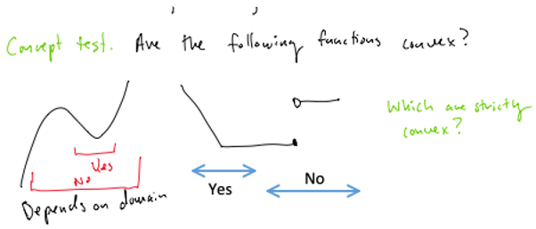
Main idea: are the objective function and feasible region both convex?

$f(x)$ is convex on the domain $x \in X$ if and only if

\alpha f(x^a) + (1 - \alpha)f(x^b) \geq f(\alpha x^a + (1 - \alpha)x^b) \quad \forall x^a, x^b \in X, \, \alpha \in (0, 1).

(4)

Strict convexity requires the inequality to be strict.

The region $\mathcal{Y}$ is convex if and only if

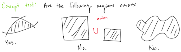
\alpha x^a + (1 - \alpha)x^b \in \mathcal{Y} \quad \forall x^a, x^b \in \mathcal{Y}, \, \alpha \in [0, 1].

(5)

Theorem 4.2: Convexity¶

Theorem 4.2 If $g(x)$ is convex and $h(x)$ is linear, then the region

\mathcal{F} = \{ x \,|\, g(x) \leq 0, h(x) = 0 \}

(6)

is convex, i.e.,

\alpha x^a + (1 - \alpha)x^b \in \mathcal{F} \quad \text{for all } \alpha \in (0, 1) \text{ and } x^a, x^b \in \mathcal{F}.

(7)

Proof

Consider two points $x^a, x^b \in \mathcal{F}$ and
$\bar{x} = \alpha x^a + (1 - \alpha)x^b \quad \text{for some } \alpha \in (0, 1).$
(8)
If $\bar{x} \not\in \mathcal{F}$ , then (i) $g(\bar{x}) > 0$ or (ii) $h(\bar{x}) \neq 0$ or both.
- Case (i): Recall $g(x)$ is convex, and $g(x^a) \leq 0$ and $g(x^b) \leq 0$ (both $x^a$ and $x^b$ are feasible).
  $0 \geq \alpha g(x^a) + (1 - \alpha)g(x^b) \geq g(\alpha x^a + (1 - \alpha)x^b) = g(\bar{x}) \quad \text{(definition of convexity)}.$
  (9)
  
  Thus, $g(\bar{x}) \leq 0$ .
- Case (ii): Recall $h(x)$ is linear, and $h(x^a) = 0$ and $h(x^b) = 0$ .
  $\begin{align*} 0 & = \alpha h(x^a) + (1 - \alpha)h(x^b) \quad \text{(property of linear functions)} \\ & = h(\alpha x^a + (1 - \alpha)x^b) = h(\bar{x}) \quad \text{(definition of } \bar{x} \text{)}. \end{align*}$
  (10)
  Thus, $g(\bar{x}) \leq 0$ and $h(\bar{x}) = 0$ .

This leads to a contradiction.

Theorem 4.3: Global Minimizers¶

Theorem 4.3 If $f(x)$ is convex and $\mathcal{F}$ is convex, then every local minimum in $\mathcal{F}$ is a global minimum. If $f(x)$ is strictly convex in $\mathcal{F}$ , then a local minimum is the unique global minimum.

Proof: Convexity Claim

Assumption: There are two local minima $x^a, x^b \in \mathcal{F}$ with $f(x^a) > f(x^b)$ . Seek contradiction.
Definition of Local Minimum:
- $f(x^a) \leq f(x), \, x \in \mathcal{N}(x^a) \cap \mathcal{F}$
- $f(x^b) \leq f(x), \, x \in \mathcal{N}(x^b) \cap \mathcal{F}$
By Convexity:
- $(1 - \alpha)x^a + \alpha x^b \in \mathcal{F}$
- $f((1 - \alpha)x^a + \alpha x^b) \leq (1 - \alpha)f(x^a) + \alpha f(x^b), \, \forall \alpha \in (0, 1)$
Choose $\alpha$ such that:
$\bar{x} = (1 - \alpha)x^a + \alpha x^b \in \mathcal{N}(x^a) \cap \mathcal{F}.$
(11)
Thus,
$f(\bar{x}) \leq f(x^a) + \alpha (f(x^b) - f(x^a)).$
(12)
Recall $f(x^b) < f(x^a)$ , so
$f(\bar{x}) < f(x^a).$
(13)
This is a contradiction, as $x^a$ cannot be a local minimizer.

Proof: Strict Convexity Claim. Same idea as above. Assume $f(x^a) \geq f(x^b)$ in (1). Use strict inequality (from the strict convexity definition) in (3) and (4).

More Illustrative Examples¶

Circle Packing Example¶

Reference: Section 4.1 in Biegler (2010)

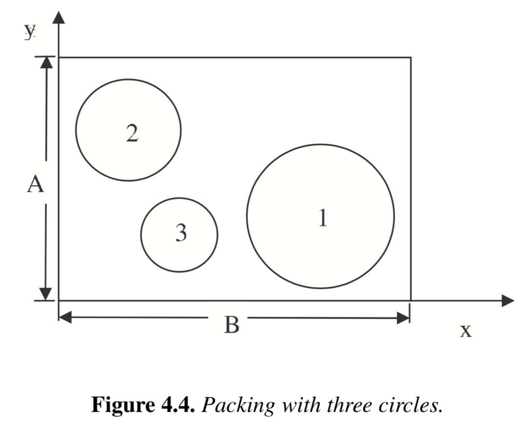
Motivating Question: Is this problem convex?

What is the smallest rectangle you can use to enclose three given circles? Reference: Example 4.4 in Biegler (2010).

Optimization Model and Pyomo Implementation¶

The following optimization model is given in Biegler (2010) and adapted to use set notation.

\begin{align*} \min_{x,y,A,B} \quad & 2(A + B) \\ \text{s.t.} \quad & A \geq 0, \quad B \geq 0 \\ & x_i, y_i \geq R_i, \quad x_i \leq B - R_i, \quad y_i \leq A - R_i, \quad \forall i \in \mathcal{C} \\ & (x_i - x_j)^2 + (y_i - y_j)^2 \geq (R_i + R_j)^2, \quad \forall i,j \in \{i \in \mathcal{C}, j \in \mathcal{C}: i < j\} \end{align*}

(14)

import matplotlib.pyplot as plt
import matplotlib.patches as mpatches


def create_circle_model(circle_radii):
    """Create circle optimization model in Pyomo

    Arguments:
        circle_radii: dictionary with keys=circle name and value=radius (float)

    Returns:
        model: Pyomo model
    """

    # Create a concrete Pyomo model.
    model = pyo.ConcreteModel()

    # Initialize index for circles
    model.CIRCLES = pyo.Set(initialize=circle_radii.keys())

    # Create parameter
    model.R = pyo.Param(
        model.CIRCLES, domain=pyo.PositiveReals, initialize=circle_radii
    )

    # Create variables for box
    model.a = pyo.Var(domain=pyo.PositiveReals)
    model.b = pyo.Var(domain=pyo.PositiveReals)

    # Set objective
    model.obj = pyo.Objective(expr=2 * (model.a + model.b), sense=pyo.minimize)

    # Create variables for circle centers
    model.x = pyo.Var(model.CIRCLES, domain=pyo.PositiveReals)
    model.y = pyo.Var(model.CIRCLES, domain=pyo.PositiveReals)

    # "In the box" constraints
    def left_x(m, c):
        return m.x[c] >= m.R[c]

    model.left_x_con = pyo.Constraint(model.CIRCLES, rule=left_x)

    def left_y(m, c):
        return m.y[c] >= m.R[c]

    model.left_y_con = pyo.Constraint(model.CIRCLES, rule=left_y)

    def right_x(m, c):
        return m.x[c] <= m.b - m.R[c]

    model.right_x_con = pyo.Constraint(model.CIRCLES, rule=right_x)

    def right_y(m, c):
        return m.y[c] <= m.a - m.R[c]

    model.right_y_con = pyo.Constraint(model.CIRCLES, rule=right_y)

    # No overlap constraints
    def no_overlap(m, c1, c2):
        if c1 < c2:
            return (m.x[c1] - m.x[c2]) ** 2 + (m.y[c1] - m.y[c2]) ** 2 >= (
                m.R[c1] + m.R[c2]
            ) ** 2
        else:
            return pyo.Constraint.Skip

    model.no_overlap_con = pyo.Constraint(model.CIRCLES, model.CIRCLES, rule=no_overlap)

    return model


def initialize_circle_model(model, a_init=25, b_init=25):
    """Initialize the x and y coordinates using uniform distribution

    Arguments:
        model: Pyomo concrete model (modified in place)
        a_init: initial value for a (default=25)
        b_init: initial value for b (default=25)

    Returns:
        Nothing. But per Pyomo scoping rules, the input argument `model`
        can be modified in this function.

    """
    # Initialize
    model.a = a_init
    model.b = b_init

    for i in model.CIRCLES:
        # Adding circle radii ensures the remains in the >0, >0 quadrant
        model.x[i] = random.uniform(0, 10) + model.R[i]
        model.y[i] = random.uniform(0, 10) + model.R[i]

Next, we will create a dictionary containing the circle names and radii values.

# Create dictionary with circle data
circle_data = {"A": 10.0, "B": 5.0, "C": 3.0}
circle_data

{'A': 10.0, 'B': 5.0, 'C': 3.0}

# Access the keys
circle_data.keys()

dict_keys(['A', 'B', 'C'])

Now let’s create the model.

# Create model
model = create_circle_model(circle_data)

And let’s initialize the model.

# Initialize model
initialize_circle_model(model)
model.pprint()

1 Set Declarations
    CIRCLES : Size=1, Index=None, Ordered=Insertion
        Key  : Dimen : Domain : Size : Members
        None :     1 :    Any :    3 : {'A', 'B', 'C'}

1 Param Declarations
    R : Size=3, Index=CIRCLES, Domain=PositiveReals, Default=None, Mutable=False
        Key : Value
          A :  10.0
          B :   5.0
          C :   3.0

4 Var Declarations
    a : Size=1, Index=None
        Key  : Lower : Value : Upper : Fixed : Stale : Domain
        None :     0 :    25 :  None : False : False : PositiveReals
    b : Size=1, Index=None
        Key  : Lower : Value : Upper : Fixed : Stale : Domain
        None :     0 :    25 :  None : False : False : PositiveReals
    x : Size=3, Index=CIRCLES
        Key : Lower : Value              : Upper : Fixed : Stale : Domain
          A :     0 : 18.444218515250483 :  None : False : False : PositiveReals
          B :     0 :  9.205715808308451 :  None : False : False : PositiveReals
          C :     0 :  8.112747213686085 :  None : False : False : PositiveReals
    y : Size=3, Index=CIRCLES
        Key : Lower : Value              : Upper : Fixed : Stale : Domain
          A :     0 : 17.579544029403024 :  None : False : False : PositiveReals
          B :     0 :  7.589167502929634 :  None : False : False : PositiveReals
          C :     0 :  7.049341374504143 :  None : False : False : PositiveReals

1 Objective Declarations
    obj : Size=1, Index=None, Active=True
        Key  : Active : Sense    : Expression
        None :   True : minimize : 2*(a + b)

5 Constraint Declarations
    left_x_con : Size=3, Index=CIRCLES, Active=True
        Key : Lower : Body : Upper : Active
          A :  10.0 : x[A] :  +Inf :   True
          B :   5.0 : x[B] :  +Inf :   True
          C :   3.0 : x[C] :  +Inf :   True
    left_y_con : Size=3, Index=CIRCLES, Active=True
        Key : Lower : Body : Upper : Active
          A :  10.0 : y[A] :  +Inf :   True
          B :   5.0 : y[B] :  +Inf :   True
          C :   3.0 : y[C] :  +Inf :   True
    no_overlap_con : Size=3, Index=CIRCLES*CIRCLES, Active=True
        Key        : Lower : Body                                : Upper : Active
        ('A', 'B') : 225.0 : (x[A] - x[B])**2 + (y[A] - y[B])**2 :  +Inf :   True
        ('A', 'C') : 169.0 : (x[A] - x[C])**2 + (y[A] - y[C])**2 :  +Inf :   True
        ('B', 'C') :  64.0 : (x[B] - x[C])**2 + (y[B] - y[C])**2 :  +Inf :   True
    right_x_con : Size=3, Index=CIRCLES, Active=True
        Key : Lower : Body              : Upper : Active
          A :  -Inf : x[A] - (b - 10.0) :   0.0 :   True
          B :  -Inf :  x[B] - (b - 5.0) :   0.0 :   True
          C :  -Inf :  x[C] - (b - 3.0) :   0.0 :   True
    right_y_con : Size=3, Index=CIRCLES, Active=True
        Key : Lower : Body              : Upper : Active
          A :  -Inf : y[A] - (a - 10.0) :   0.0 :   True
          B :  -Inf :  y[B] - (a - 5.0) :   0.0 :   True
          C :  -Inf :  y[C] - (a - 3.0) :   0.0 :   True

12 Declarations: CIRCLES R a b obj x y left_x_con left_y_con right_x_con right_y_con no_overlap_con

Visualize Initial Point¶

Next, we’ll define a function to plot the solution (or initial point)

# Plot initial point


def plot_circles(m):
    """Plot circles using data in Pyomo model

    Arguments:
        m: Pyomo concrete model

    Returns:
        Nothing (but makes a figure)

    """

    # Create figure
    fig, ax = plt.subplots(1, figsize=(6, 6))

    # Adjust axes
    l = max(m.a.value, m.b.value) + 1
    ax.set_xlim(0, l)
    ax.set_ylim(0, l)

    # Draw box
    art = mpatches.Rectangle((0, 0), width=m.b.value, height=m.a.value, fill=False)
    ax.add_patch(art)

    # Draw circles and mark center
    for i in m.CIRCLES:
        art2 = mpatches.Circle(
            (m.x[i].value, m.y[i].value), radius=m.R[i], fill=True, alpha=0.25
        )
        ax.add_patch(art2)

        plt.scatter(m.x[i].value, m.y[i].value, color="black")

    # Show plot
    plt.show()


plot_circles(model)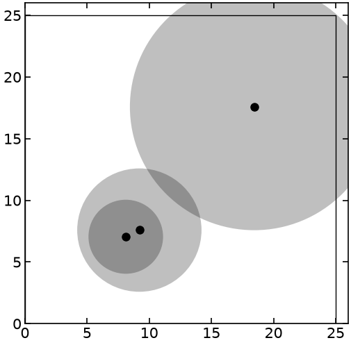

Solve and Inspect the Solution¶

# Specify the solver
solver = pyo.SolverFactory("ipopt")

# Solve the model
results = solver.solve(model, tee=True)
assert pyo.check_optimal_termination(results), (
    f"Solve failed: status={results.solver.status}, "
    f"termination={results.solver.termination_condition}"
)

Ipopt 3.13.2: 

******************************************************************************
This program contains Ipopt, a library for large-scale nonlinear optimization.
 Ipopt is released as open source code under the Eclipse Public License (EPL).
         For more information visit http://projects.coin-or.org/Ipopt

This version of Ipopt was compiled from source code available at
    https://github.com/IDAES/Ipopt as part of the Institute for the Design of
    Advanced Energy Systems Process Systems Engineering Framework (IDAES PSE
    Framework) Copyright (c) 2018-2019. See https://github.com/IDAES/idaes-pse.

This version of Ipopt was compiled using HSL, a collection of Fortran codes
    for large-scale scientific computation.  All technical papers, sales and
    publicity material resulting from use of the HSL codes within IPOPT must
    contain the following acknowledgement:
        HSL, a collection of Fortran codes for large-scale scientific
        computation. See http://www.hsl.rl.ac.uk.
******************************************************************************

This is Ipopt version 3.13.2, running with linear solver ma27.

Number of nonzeros in equality constraint Jacobian...:        0
Number of nonzeros in inequality constraint Jacobian.:       30
Number of nonzeros in Lagrangian Hessian.............:       12

Total number of variables............................:        8
                     variables with only lower bounds:        8
                variables with lower and upper bounds:        0
                     variables with only upper bounds:        0
Total number of equality constraints.................:        0
Total number of inequality constraints...............:       15
        inequality constraints with only lower bounds:        9
   inequality constraints with lower and upper bounds:        0
        inequality constraints with only upper bounds:        6

iter    objective    inf_pr   inf_du lg(mu)  ||d||  lg(rg) alpha_du alpha_pr  ls
   0  1.0000000e+02 6.25e+01 1.05e+00  -1.0 0.00e+00    -  0.00e+00 0.00e+00   0
   1  1.0046267e+02 4.59e+01 1.05e+01  -1.0 2.67e+01   0.0 1.52e-01 5.64e-02h  1
   2  1.0446269e+02 2.46e+01 2.54e+00  -1.0 5.43e+00  -0.5 5.62e-01 3.57e-01h  1
   3  1.1075999e+02 0.00e+00 4.40e+00  -1.0 4.83e+00  -1.0 6.87e-01 1.00e+00h  1
   4  1.0931790e+02 0.00e+00 4.22e+00  -1.0 6.13e+01  -1.4 3.27e-01 2.76e-02f  3
   5  1.0505265e+02 0.00e+00 8.83e-01  -1.0 2.84e+00  -1.0 1.00e+00 9.20e-01f  1
   6  1.0163361e+02 0.00e+00 1.15e+00  -1.0 1.96e+00  -1.5 4.90e-01 9.10e-01h  1
   7  9.9775211e+01 0.00e+00 1.90e-01  -1.0 2.12e+00  -1.1 1.00e+00 8.60e-01f  1
   8  9.8947266e+01 0.00e+00 8.86e-01  -1.0 1.23e+02    -  3.86e-01 5.70e-02f  1
   9  9.8937271e+01 0.00e+00 2.06e-02  -1.0 7.04e-01  -1.5 1.00e+00 1.00e+00h  1
iter    objective    inf_pr   inf_du lg(mu)  ||d||  lg(rg) alpha_du alpha_pr  ls
  10  9.8325956e+01 0.00e+00 6.43e-03  -2.5 3.75e+00    -  9.93e-01 9.37e-01f  1
  11  9.8301250e+01 0.00e+00 2.66e-03  -2.5 4.81e+01    -  4.81e-01 1.00e+00h  1
  12  9.8301257e+01 0.00e+00 5.36e-04  -2.5 2.99e+01    -  1.00e+00 1.00e+00h  1
  13  9.8301256e+01 0.00e+00 2.96e-05  -2.5 2.59e+01    -  1.00e+00 1.00e+00h  1
  14  9.8301256e+01 0.00e+00 1.40e-06  -2.5 2.48e+00    -  1.00e+00 1.00e+00h  1
  15  9.8285159e+01 0.00e+00 2.69e-07  -3.8 3.80e-02    -  1.00e+00 1.00e+00h  1
  16  9.8284281e+01 0.00e+00 9.89e-10  -5.7 2.05e-03    -  1.00e+00 1.00e+00h  1
  17  9.8284270e+01 0.00e+00 9.89e-13  -8.6 1.62e-04    -  1.00e+00 1.00e+00h  1

Number of Iterations....: 17

                                   (scaled)                 (unscaled)
Objective...............:   9.8284270438747257e+01    9.8284270438747257e+01
Dual infeasibility......:   9.8878042122038317e-13    9.8878042122038317e-13
Constraint violation....:   0.0000000000000000e+00    0.0000000000000000e+00
Complementarity.........:   2.5165074041737747e-09    2.5165074041737747e-09
Overall NLP error.......:   2.5165074041737747e-09    2.5165074041737747e-09


Number of objective function evaluations             = 22
Number of objective gradient evaluations             = 18
Number of equality constraint evaluations            = 0
Number of inequality constraint evaluations          = 22
Number of equality constraint Jacobian evaluations   = 0
Number of inequality constraint Jacobian evaluations = 18
Number of Lagrangian Hessian evaluations             = 17
Total CPU secs in IPOPT (w/o function evaluations)   =      0.002
Total CPU secs in NLP function evaluations           =      0.000

EXIT: Optimal Solution Found.

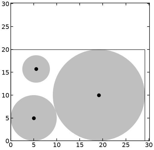
Next, we can inspect the solution. Because Pyomo is a Python extension, we can use Python (for loops, etc.) to programmatically inspect the solution.

# Print variable values
print("Name\tValue")
for c in model.component_data_objects(pyo.Var):
    print(c.name, "\t", pyo.value(c))

# Plot solution
plot_circles(model)

Name	Value
a 	 19.999999803189603
b 	 29.14213541618403
x[A] 	 19.14213551493119
x[B] 	 4.999999951252128
x[C] 	 5.517274811159322
y[A] 	 9.999999901937443
y[B] 	 4.999999953543125
y[C] 	 15.729315741741758

# Print constraints
for c in model.component_data_objects(pyo.Constraint):
    print(
        c.name,
        "\t",
        pyo.value(c.lower),
        "\t",
        pyo.value(c.body),
        "\t",
        pyo.value(c.upper),
    )

left_x_con[A] 	 10.0 	 19.14213551493119 	 None
left_x_con[B] 	 5.0 	 4.999999951252128 	 None
left_x_con[C] 	 3.0 	 5.517274811159322 	 None
left_y_con[A] 	 10.0 	 9.999999901937443 	 None
left_y_con[B] 	 5.0 	 4.999999953543125 	 None
left_y_con[C] 	 3.0 	 15.729315741741758 	 None
right_x_con[A] 	 None 	 9.87471615587765e-08 	 0.0
right_x_con[B] 	 None 	 -19.1421354649319 	 0.0
right_x_con[C] 	 None 	 -20.624860605024708 	 0.0
right_y_con[A] 	 None 	 9.874784012708915e-08 	 0.0
right_y_con[B] 	 None 	 -9.999999849646478 	 0.0
right_y_con[C] 	 None 	 -1.2706840614478452 	 0.0
no_overlap_con[A,B] 	 225.0 	 224.99999778541928 	 None
no_overlap_con[A,C] 	 169.0 	 218.46188918941948 	 None
no_overlap_con[B,C] 	 64.0 	 115.38579056358046 	 None

Reinitialize and Resolve¶

Reinitialize the model, plot the initial point, resolve, and plot the solution. Is there more than one solution?

# Initialize and print the model
initialize_circle_model(model)

# Plot initial point
plot_circles(model)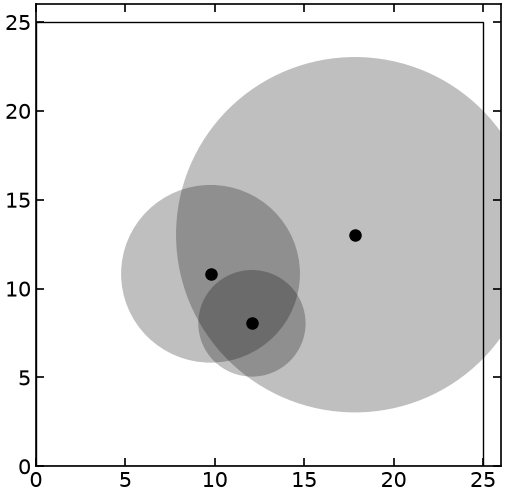

# Solve the model
results = solver.solve(model, tee=True)
assert pyo.check_optimal_termination(results), (
    f"Solve failed: status={results.solver.status}, "
    f"termination={results.solver.termination_condition}"
)

Ipopt 3.13.2: 

******************************************************************************
This program contains Ipopt, a library for large-scale nonlinear optimization.
 Ipopt is released as open source code under the Eclipse Public License (EPL).
         For more information visit http://projects.coin-or.org/Ipopt

This version of Ipopt was compiled from source code available at
    https://github.com/IDAES/Ipopt as part of the Institute for the Design of
    Advanced Energy Systems Process Systems Engineering Framework (IDAES PSE
    Framework) Copyright (c) 2018-2019. See https://github.com/IDAES/idaes-pse.

This version of Ipopt was compiled using HSL, a collection of Fortran codes
    for large-scale scientific computation.  All technical papers, sales and
    publicity material resulting from use of the HSL codes within IPOPT must
    contain the following acknowledgement:
        HSL, a collection of Fortran codes for large-scale scientific
        computation. See http://www.hsl.rl.ac.uk.
******************************************************************************

This is Ipopt version 3.13.2, running with linear solver ma27.

Number of nonzeros in equality constraint Jacobian...:        0
Number of nonzeros in inequality constraint Jacobian.:       30
Number of nonzeros in Lagrangian Hessian.............:       12

Total number of variables............................:        8
                     variables with only lower bounds:        8
                variables with lower and upper bounds:        0
                     variables with only upper bounds:        0
Total number of equality constraints.................:        0
Total number of inequality constraints...............:       15
        inequality constraints with only lower bounds:        9
   inequality constraints with lower and upper bounds:        0
        inequality constraints with only upper bounds:        6

iter    objective    inf_pr   inf_du lg(mu)  ||d||  lg(rg) alpha_du alpha_pr  ls
   0  1.0000000e+02 1.55e+02 1.00e+00  -1.0 0.00e+00    -  0.00e+00 0.00e+00   0
   1  1.0138375e+02 9.34e+01 7.73e-01  -1.0 1.19e+01    -  4.61e-01 3.31e-01h  1
   2  9.9526817e+01 4.07e+01 5.97e-01  -1.0 3.04e+01  -2.0 2.98e-01 1.77e-01h  1
   3  9.8395427e+01 2.47e+01 4.51e-01  -1.0 3.49e+00    -  9.69e-01 3.60e-01h  1
   4  9.8926255e+01 1.22e-01 9.29e-02  -1.0 3.37e+00    -  7.52e-01 8.39e-01h  1
   5  9.8741856e+01 5.57e-02 1.63e-01  -1.0 1.62e+02    -  7.54e-01 3.84e-01f  1
   6  9.8917368e+01 0.00e+00 3.14e-03  -1.0 3.30e+01    -  1.00e+00 1.00e+00h  1
   7  9.8900000e+01 0.00e+00 1.04e-03  -1.0 7.91e+00    -  1.00e+00 1.00e+00h  1
   8  9.8394513e+01 0.00e+00 4.20e-04  -1.7 1.76e+00    -  1.00e+00 1.00e+00h  1
   9  9.8284893e+01 0.00e+00 4.60e-05  -3.8 2.95e-01    -  1.00e+00 9.98e-01h  1
iter    objective    inf_pr   inf_du lg(mu)  ||d||  lg(rg) alpha_du alpha_pr  ls
  10  9.8284281e+01 0.00e+00 5.07e-08  -5.7 5.23e-02    -  1.00e+00 1.00e+00h  1
  11  9.8284270e+01 0.00e+00 3.77e-11  -8.6 4.78e-03    -  1.00e+00 1.00e+00h  1

Number of Iterations....: 11

                                   (scaled)                 (unscaled)
Objective...............:   9.8284270438748450e+01    9.8284270438748450e+01
Dual infeasibility......:   3.7706208248288032e-11    3.7706208248288032e-11
Constraint violation....:   0.0000000000000000e+00    0.0000000000000000e+00
Complementarity.........:   2.7106270175648520e-09    2.7106270175648520e-09
Overall NLP error.......:   2.7106270175648520e-09    2.7106270175648520e-09


Number of objective function evaluations             = 12
Number of objective gradient evaluations             = 12
Number of equality constraint evaluations            = 0
Number of inequality constraint evaluations          = 12
Number of equality constraint Jacobian evaluations   = 0
Number of inequality constraint Jacobian evaluations = 12
Number of Lagrangian Hessian evaluations             = 11
Total CPU secs in IPOPT (w/o function evaluations)   =      0.001
Total CPU secs in NLP function evaluations           =      0.000

EXIT: Optimal Solution Found.

# Plot solution
plot_circles(model)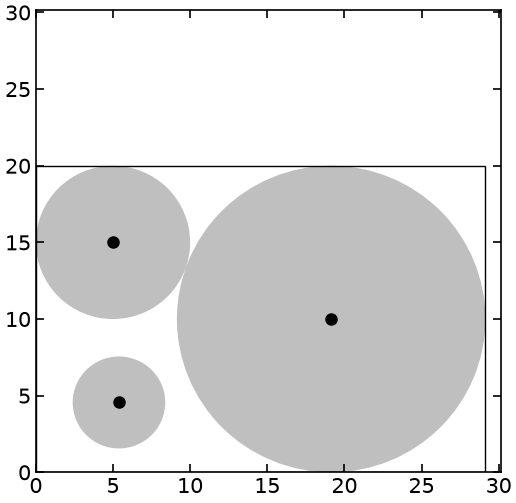

Take Away Messages¶

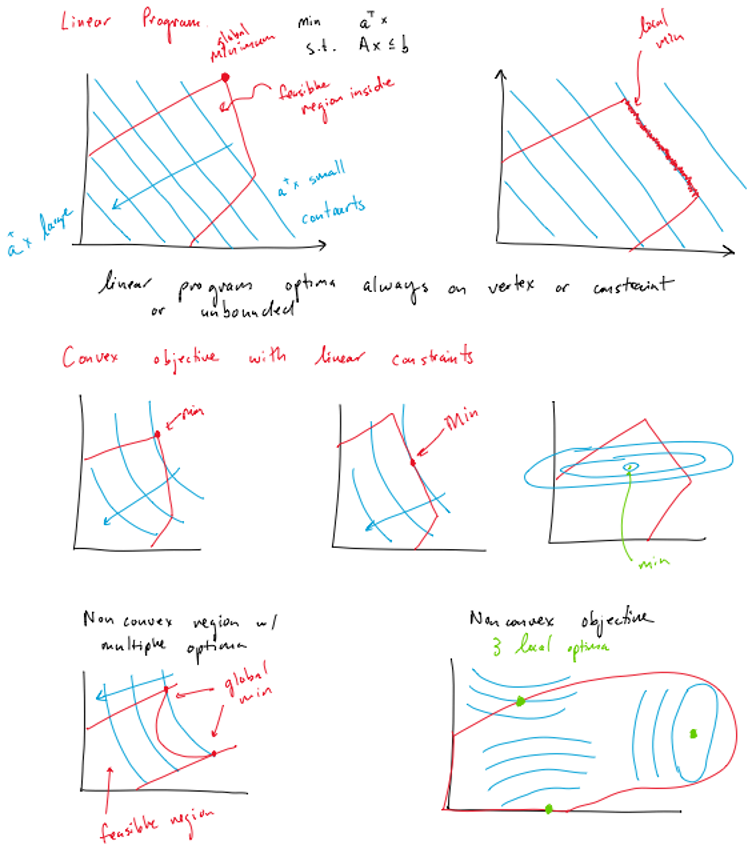
Nonlinear programs may be nonconvex. For nonconvex problems, there often exist many local optima that are not also global optima.
Initialization is really important in optimization problems with nonlinear objectives or constraints!