# This code cell installs packages on Colab

import sys

if "google.colab" in sys.modules:
    !wget "https://raw.githubusercontent.com/ndcbe/optimization/main/notebooks/helper.py"
    import helper

    helper.easy_install()
else:
    sys.path.insert(0, "../")
    import helper
helper.set_plotting_style()

# `helper` is the ONE course module: the Colab install above, the house figure
# style, and the extract / archive / save-the-figure plumbing this notebook uses
# further down. It used to take a second `wget` for `pyomo_results.py`; that
# module is now a shim over this one, and one file is one thing that can fail.
import random

import pandas as pd
import matplotlib.pyplot as plt
import matplotlib.patches as mpatches
import pyomo.environ as pyo

# Seed the random number generator so this notebook is reproducible
# (Pyomo style guide, section 8).
random.seed(0)
Nonlinear Programs: Circle Packing Example
What is the smallest rectangle you can use to enclose three given circles? Reference: Example 4.4 in Biegler (2010).
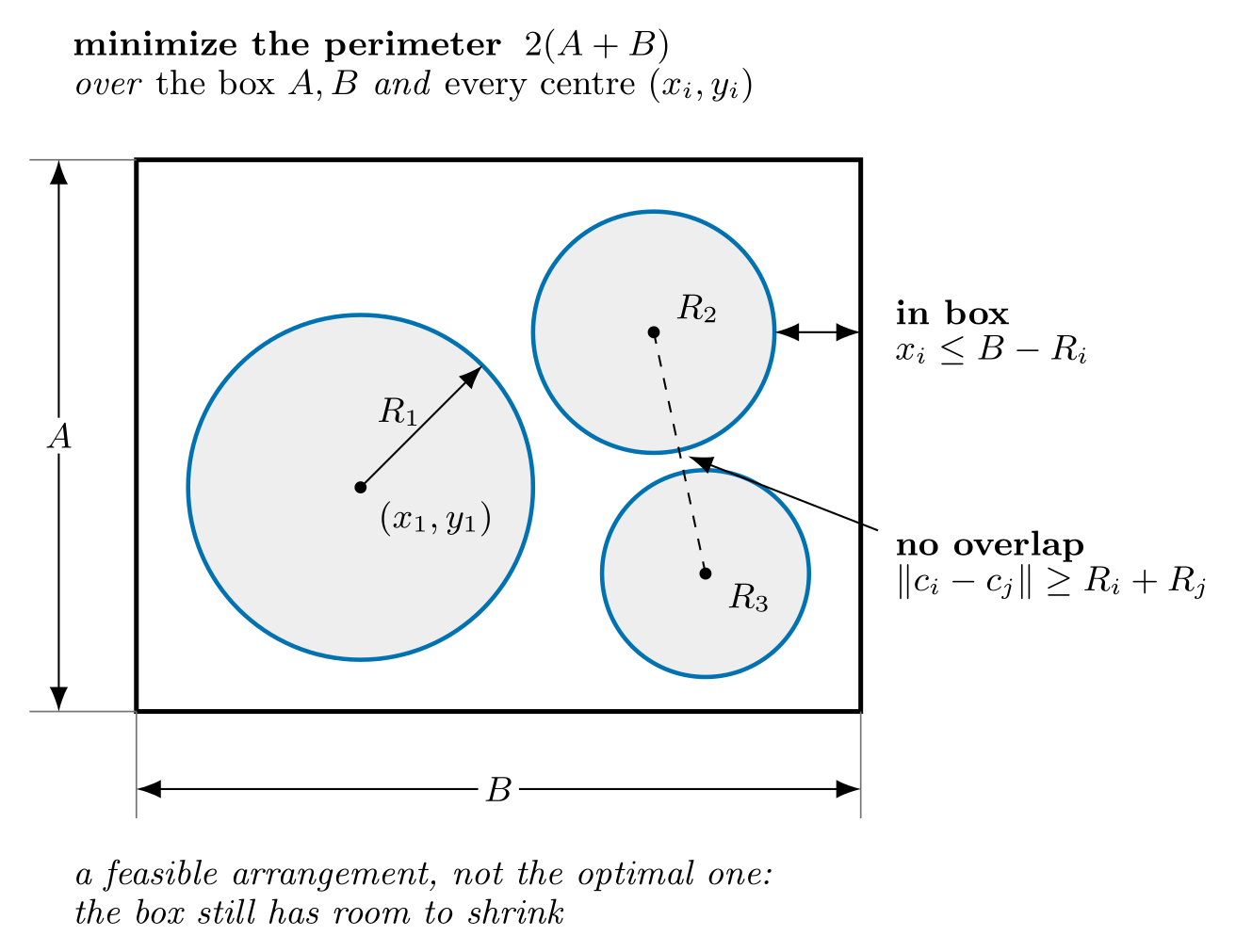
This is the same illustration the lecture handout prints. It is drawn once, in
figures/tikz/circle-packing-problem.tex, and rendered for both the website and the
course pack, so the picture on this page and the picture in your notes cannot drift apart.
Propose an Optimization Model
The following optimization model is given in Biegler (2010):
How can we more compactly represent this using sets?
Activity
Identify the sets, parameters, variables, and constraints.Sets
Click to expand
: circles
Parameters
Click to expand
: radius of circle
Variables
Click to expand
, : coordinates for circle
, : dimensions of the bounding rectangle
Objective
Click to expand
: perimeter of the bounding rectangle
Constraints
Click to expand
circle cannot overlap with sides of bounding rectangle:
no overlap between circles and :
non-negative rectangle lengths:
Complete Optimization Formulation
Click to see the solution to the activity
Activity
Perform degree of freedom analysis.Degree of Freedom Analysis
Click to expand
Continuous variables: (the box dimensions and , plus a center for each circle)
Inequality constraints:
Implement in Pyomo
First, we will define a function that builds the model.
def create_circle_model(circle_radii):
    """Create circle optimization model in Pyomo

    Arguments:
        circle_radii: dictionary with keys=circle name and value=radius (float)

    Returns:
        model: Pyomo model
    """

    # Create a concrete Pyomo model.
    model = pyo.ConcreteModel()

    # Set of circles to pack, C in the notes
    model.CIRCLES = pyo.Set(initialize=circle_radii.keys())

    # Radius of each circle, R_i in the notes [m].
    # initialize= supplies the data; domain= is checked when it is loaded.
    model.R = pyo.Param(
        model.CIRCLES,
        domain=pyo.PositiveReals,
        initialize=circle_radii,
        units=pyo.units.m,
    )

    # Height of the enclosing box, A in the notes [m]
    model.box_height = pyo.Var(domain=pyo.PositiveReals, units=pyo.units.m)

    # Width of the enclosing box, B in the notes [m]
    model.box_width = pyo.Var(domain=pyo.PositiveReals, units=pyo.units.m)

    # Center of circle i, (x_i, y_i) in the notes [m].
    # A DOMAIN (or bounds=) is not a constraint: it is handled directly by the
    # solver's bound machinery, which is cheaper than a general inequality row.
    # Prefer it whenever the restriction is a simple bound on one variable.
    model.x = pyo.Var(model.CIRCLES, domain=pyo.PositiveReals, units=pyo.units.m)
    model.y = pyo.Var(model.CIRCLES, domain=pyo.PositiveReals, units=pyo.units.m)

    # Minimize the perimeter of the box [m]
    model.obj = pyo.Objective(
        expr=2 * (model.box_height + model.box_width), sense=pyo.minimize
    )

    # "In the box" constraints. The decorated rule receives the block as its
    # first argument, so `b` is the model being built.
    #
    # ONE declaration, MANY constraints: @model.Constraint(model.CIRCLES) calls
    # the function once per member of CIRCLES. That is the "for all i in C" of
    # the written model.
    #
    # The rule RETURNS AN EXPRESSION, not a number. b.x[c] is a variable
    # object, so `>=` between Pyomo objects builds a relation rather than
    # evaluating a comparison to True or False.
    @model.Constraint(model.CIRCLES)
    def left_x_con(b, c):
        """Keep circle c inside the left edge of the box."""
        return b.x[c] >= b.R[c]

    @model.Constraint(model.CIRCLES)
    def left_y_con(b, c):
        """Keep circle c above the bottom edge of the box."""
        return b.y[c] >= b.R[c]

    @model.Constraint(model.CIRCLES)
    def right_x_con(b, c):
        """Keep circle c inside the right edge of the box."""
        return b.x[c] <= b.box_width - b.R[c]

    @model.Constraint(model.CIRCLES)
    def right_y_con(b, c):
        """Keep circle c below the top edge of the box."""
        return b.y[c] <= b.box_height - b.R[c]

    # No overlap constraints, declared over CIRCLES x CIRCLES. Returning
    # Constraint.Skip omits a member of the index set, which is how a rule over
    # the full product becomes one constraint per pair with c1 < c2 -- half the
    # square, and no self-pairs.
    @model.Constraint(model.CIRCLES, model.CIRCLES)
    def no_overlap_con(b, c1, c2):
        """Separate each distinct pair of circles."""
        if c1 < c2:
            return (b.x[c1] - b.x[c2]) ** 2 + (b.y[c1] - b.y[c2]) ** 2 >= (
                b.R[c1] + b.R[c2]
            ) ** 2
        else:
            return pyo.Constraint.Skip

    return model
Next, we will define a function that initializes the model. Notice this is separate from the function above: the model and the initial point are two different things, and for a nonconvex problem the initial point is part of the specification of what you solved.
def initialize_circle_model(model, height_init=25, width_init=25, spread=10):
    """Initialize the x and y coordinates using uniform distribution

    Arguments:
        model: Pyomo model
        height_init: initial value for box_height (default=25)
        width_init: initial value for box_width (default=25)
        spread: width of the uniform window the centers are drawn from
            (default=10)

    Returns:
        Nothing. But per Pyomo scoping rules, the input argument `model`
        can be modified in this function.

    """
    # Initialize
    model.box_height = height_init
    model.box_width = width_init

    for i in model.CIRCLES:
        # Adding circle radii ensures the circle remains in the >0, >0 quadrant
        model.x[i] = random.uniform(0, spread) + pyo.value(model.R[i])
        model.y[i] = random.uniform(0, spread) + pyo.value(model.R[i])
Next, we will create a dictionary containing the circle names and radii values.
# Create dictionary with circle data
circle_data = {"A": 10.0, "B": 5.0, "C": 3.0}
circle_data
{'A': 10.0, 'B': 5.0, 'C': 3.0}# Access the keys
circle_data.keys()dict_keys(['A', 'B', 'C'])Now let’s create the model.
# Create model
model = create_circle_model(circle_data)
model.pprint()
1 Set Declarations
CIRCLES : Size=1, Index=None, Ordered=Insertion
Key : Dimen : Domain : Size : Members
None : 1 : Any : 3 : {'A', 'B', 'C'}
1 Param Declarations
R : Size=3, Index=CIRCLES, Domain=PositiveReals, Default=None, Mutable=True, Units=m
Key : Value
A : 10.0
B : 5.0
C : 3.0
4 Var Declarations
box_height : Size=1, Index=None, Units=m
Key : Lower : Value : Upper : Fixed : Stale : Domain
None : 0 : None : None : False : True : PositiveReals
box_width : Size=1, Index=None, Units=m
Key : Lower : Value : Upper : Fixed : Stale : Domain
None : 0 : None : None : False : True : PositiveReals
x : Size=3, Index=CIRCLES, Units=m
Key : Lower : Value : Upper : Fixed : Stale : Domain
A : 0 : None : None : False : True : PositiveReals
B : 0 : None : None : False : True : PositiveReals
C : 0 : None : None : False : True : PositiveReals
y : Size=3, Index=CIRCLES, Units=m
Key : Lower : Value : Upper : Fixed : Stale : Domain
A : 0 : None : None : False : True : PositiveReals
B : 0 : None : None : False : True : PositiveReals
C : 0 : None : None : False : True : PositiveReals
1 Objective Declarations
obj : Size=1, Index=None, Active=True
Key : Active : Sense : Expression
None : True : minimize : 2*(box_height + box_width)
5 Constraint Declarations
left_x_con : Size=3, Index=CIRCLES, Active=True
Key : Lower : Body : Upper : Active
A : R[A] : x[A] : +Inf : True
B : R[B] : x[B] : +Inf : True
C : R[C] : x[C] : +Inf : True
left_y_con : Size=3, Index=CIRCLES, Active=True
Key : Lower : Body : Upper : Active
A : R[A] : y[A] : +Inf : True
B : R[B] : y[B] : +Inf : True
C : R[C] : y[C] : +Inf : True
no_overlap_con : Size=3, Index=CIRCLES*CIRCLES, Active=True
Key : Lower : Body : Upper : Active
('A', 'B') : (R[A] + R[B])**2 : (x[A] - x[B])**2 + (y[A] - y[B])**2 : +Inf : True
('A', 'C') : (R[A] + R[C])**2 : (x[A] - x[C])**2 + (y[A] - y[C])**2 : +Inf : True
('B', 'C') : (R[B] + R[C])**2 : (x[B] - x[C])**2 + (y[B] - y[C])**2 : +Inf : True
right_x_con : Size=3, Index=CIRCLES, Active=True
Key : Lower : Body : Upper : Active
A : -Inf : x[A] - (box_width - R[A]) : 0.0 : True
B : -Inf : x[B] - (box_width - R[B]) : 0.0 : True
C : -Inf : x[C] - (box_width - R[C]) : 0.0 : True
right_y_con : Size=3, Index=CIRCLES, Active=True
Key : Lower : Body : Upper : Active
A : -Inf : y[A] - (box_height - R[A]) : 0.0 : True
B : -Inf : y[B] - (box_height - R[B]) : 0.0 : True
C : -Inf : y[C] - (box_height - R[C]) : 0.0 : True
12 Declarations: CIRCLES R box_height box_width x y obj left_x_con left_y_con right_x_con right_y_con no_overlap_con
The radii and the coordinates are declared in metres with units=pyo.units.m, so Pyomo can check that every constraint and the objective are dimensionally consistent. Run that check before handing the model to a solver: it catches a whole class of modeling mistake that a solver will happily converge on.
from pyomo.util.check_units import assert_units_consistent

# Raises InconsistentUnitsError if any constraint or the objective mixes units
assert_units_consistent(model)
print("Units are consistent.")
Units are consistent.
And let’s initialize the model.
# Initialize model
initialize_circle_model(model)
model.pprint()
1 Set Declarations
CIRCLES : Size=1, Index=None, Ordered=Insertion
Key : Dimen : Domain : Size : Members
None : 1 : Any : 3 : {'A', 'B', 'C'}
1 Param Declarations
R : Size=3, Index=CIRCLES, Domain=PositiveReals, Default=None, Mutable=True, Units=m
Key : Value
A : 10.0
B : 5.0
C : 3.0
4 Var Declarations
box_height : Size=1, Index=None, Units=m
Key : Lower : Value : Upper : Fixed : Stale : Domain
None : 0 : 25 : None : False : False : PositiveReals
box_width : Size=1, Index=None, Units=m
Key : Lower : Value : Upper : Fixed : Stale : Domain
None : 0 : 25 : None : False : False : PositiveReals
x : Size=3, Index=CIRCLES, Units=m
Key : Lower : Value : Upper : Fixed : Stale : Domain
A : 0 : 18.444218515250483 : None : False : False : PositiveReals
B : 0 : 9.205715808308451 : None : False : False : PositiveReals
C : 0 : 8.112747213686085 : None : False : False : PositiveReals
y : Size=3, Index=CIRCLES, Units=m
Key : Lower : Value : Upper : Fixed : Stale : Domain
A : 0 : 17.579544029403024 : None : False : False : PositiveReals
B : 0 : 7.589167502929634 : None : False : False : PositiveReals
C : 0 : 7.049341374504143 : None : False : False : PositiveReals
1 Objective Declarations
obj : Size=1, Index=None, Active=True
Key : Active : Sense : Expression
None : True : minimize : 2*(box_height + box_width)
5 Constraint Declarations
left_x_con : Size=3, Index=CIRCLES, Active=True
Key : Lower : Body : Upper : Active
A : R[A] : x[A] : +Inf : True
B : R[B] : x[B] : +Inf : True
C : R[C] : x[C] : +Inf : True
left_y_con : Size=3, Index=CIRCLES, Active=True
Key : Lower : Body : Upper : Active
A : R[A] : y[A] : +Inf : True
B : R[B] : y[B] : +Inf : True
C : R[C] : y[C] : +Inf : True
no_overlap_con : Size=3, Index=CIRCLES*CIRCLES, Active=True
Key : Lower : Body : Upper : Active
('A', 'B') : (R[A] + R[B])**2 : (x[A] - x[B])**2 + (y[A] - y[B])**2 : +Inf : True
('A', 'C') : (R[A] + R[C])**2 : (x[A] - x[C])**2 + (y[A] - y[C])**2 : +Inf : True
('B', 'C') : (R[B] + R[C])**2 : (x[B] - x[C])**2 + (y[B] - y[C])**2 : +Inf : True
right_x_con : Size=3, Index=CIRCLES, Active=True
Key : Lower : Body : Upper : Active
A : -Inf : x[A] - (box_width - R[A]) : 0.0 : True
B : -Inf : x[B] - (box_width - R[B]) : 0.0 : True
C : -Inf : x[C] - (box_width - R[C]) : 0.0 : True
right_y_con : Size=3, Index=CIRCLES, Active=True
Key : Lower : Body : Upper : Active
A : -Inf : y[A] - (box_height - R[A]) : 0.0 : True
B : -Inf : y[B] - (box_height - R[B]) : 0.0 : True
C : -Inf : y[C] - (box_height - R[C]) : 0.0 : True
12 Declarations: CIRCLES R box_height box_width x y obj left_x_con left_y_con right_x_con right_y_con no_overlap_con
Activity
Compare the initial values forx and y with and without initialization. What is the default initial value in Pyomo?Visualize Initial Point
Next we define the function that draws an arrangement of circles. Two things about it are worth copying into your own work.
It takes extracted results, not the Pyomo model. extract_circles turns the model
into plain Python; plot_circles draws that plain Python and never sees the model. So
you can fiddle with the picture as many times as you like without calling Ipopt again,
and the picture cannot quietly show you something other than what you solved. The
handout figure further down is built the same way.
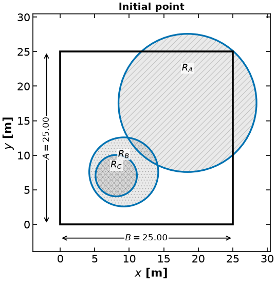
It is drawn in the course house style, the same style the lecture notes use: the box carries its two dimensions and (those are the objective), each circle is labelled with its radius, and the starting arrangement can be drawn underneath as a dotted outline. The three circles are also given three different hatch textures, so the figure still reads when it is printed in black and white.
# ---------- EXTRACT, then PLOT --------------------------------------------
# Two functions, deliberately separate -- see the note above.


def extract_circles(m):
    """Pyomo model -> plain Python. After this, nothing needs the model again.

    Arguments:
        m: Pyomo concrete model, solved or merely initialized

    Returns:
        dict with the box dimensions `A` and `B`, the `radii`, and the `centers`
    """
    return {
        "A": pyo.value(m.box_height),
        "B": pyo.value(m.box_width),
        "radii": {i: pyo.value(m.R[i]) for i in m.CIRCLES},
        "centers": {i: (pyo.value(m.x[i]), pyo.value(m.y[i])) for i in m.CIRCLES},
    }


# The house hatch sequence, copied from figures/plots/_house.py as a LITERAL:
# that module is not on disk on Colab, so it must not be imported here. The
# first three entries are three different texture FAMILIES -- lines, dots,
# crosses -- so every pair of circles differs in kind rather than in the sign
# of a slope, which is the cue that survives greyscale printing.
HATCHES = ("///", "...", "xxx", "|||", "---", "\\\\\\")
SHADE_ALPHA = 0.18
OKABE_BLUE = "#0072B2"  # Okabe-Ito; the only color in the figure


def plot_circles(results, start=None, title=None, ax=None, span=None):
    """Draw one arrangement of circles in a box, in the course house style.

    Arguments:
        results: dict from `extract_circles` -- the arrangement to draw solid
        start: optionally, another such dict, drawn dotted and unfilled
            underneath to show where the solver started
        title: text above the panel
        ax: draw into an existing axes instead of creating a figure
        span: force the axis range instead of computing it from the content.
            Pass the same value to several panels when their sizes are meant
            to be compared by eye -- otherwise each panel is scaled to fit and
            two boxes of different size look identical.

    Returns:
        The matplotlib Axes.
    """
    A, B = results["A"], results["B"]
    radii, centers = results["radii"], results["centers"]

    if ax is None:
        _, ax = plt.subplots(figsize=(6, 6))
    hatch_colour = plt.rcParams["hatch.color"]

    # Axis limits from the CONTENT, not from the box: at a loose initial point
    # a circle can stick out well past the walls, and clipping it hides the
    # very thing the picture is being drawn to show.
    extent = []
    for d in (results, start):
        if d is not None:
            extent += [d["A"], d["B"]]
            for i in d["radii"]:
                cx, cy = d["centers"][i]
                extent += [cx + d["radii"][i], cy + d["radii"][i]]
    span = max(extent) if span is None else span
    pad = 0.14 * span

    # Where the solver started: dotted, unfilled, underneath everything else.
    if start is not None:
        ax.add_patch(
            mpatches.Rectangle(
                (0, 0), start["B"], start["A"], facecolor="none",
                edgecolor="0.72", linestyle=":", linewidth=1.5, zorder=1,
            )
        )
        for i in start["radii"]:
            cx, cy = start["centers"][i]
            ax.add_patch(
                mpatches.Circle(
                    (cx, cy), start["radii"][i], facecolor="none",
                    edgecolor="0.72", linestyle=":", linewidth=1.5, zorder=1,
                )
            )

    # The circles: a pale hatch that survives greyscale, a blue outline, and
    # the radius written in the middle. Circle i is labelled R_i, exactly as
    # the model indexes it.
    for k, i in enumerate(radii):
        cx, cy = centers[i]
        ax.add_patch(
            mpatches.Circle(
                (cx, cy), radii[i], facecolor="0.55", alpha=SHADE_ALPHA,
                hatch=HATCHES[k % len(HATCHES)], edgecolor=hatch_colour,
                linewidth=0.0, zorder=2,
            )
        )
        ax.add_patch(
            mpatches.Circle(
                (cx, cy), radii[i], facecolor="none", edgecolor=OKABE_BLUE,
                linewidth=2.4, zorder=3,
            )
        )
        # The label sits half a radius ABOVE the center, not on it. At a loose
        # initial point two circles can be nearly concentric -- the circles
        # overlap, because an initial point need not be feasible -- and two
        # labels on the same spot are unreadable. Offsetting by a fraction of
        # each circle's OWN radius separates them, because the radii differ.
        # The white box keeps the text legible over the hatching.
        ax.annotate(
            f"$R_{{{i}}}$", xy=(cx, cy + 0.5 * radii[i]), fontsize=13,
            ha="center", va="center", zorder=6,
            bbox=dict(facecolor="white", edgecolor="none", alpha=0.75, pad=1.0),
        )

    # The box, with its two dimensions written on it: A and B ARE the objective.
    ax.add_patch(
        mpatches.Rectangle((0, 0), B, A, facecolor="none", edgecolor="black",
                           linewidth=2.6, zorder=4)
    )
    off = -0.5 * pad
    ax.annotate("", xy=(off, 0), xytext=(off, A),
                arrowprops=dict(arrowstyle="<->", color="black", lw=1.3))
    ax.annotate(f"$A = {A:.2f}$", xy=(off, 0.5 * A), fontsize=12.5, ha="center",
                va="center", rotation=90,
                bbox=dict(facecolor="white", edgecolor="none", pad=1.0))
    ax.annotate("", xy=(0, off), xytext=(B, off),
                arrowprops=dict(arrowstyle="<->", color="black", lw=1.3))
    ax.annotate(f"$B = {B:.2f}$", xy=(0.5 * B, off), fontsize=12.5, ha="center",
                va="center", bbox=dict(facecolor="white", edgecolor="none", pad=1.0))

    ax.set_xlim(-pad, span + 0.5 * pad)
    ax.set_ylim(-pad, span + 0.5 * pad)
    ax.set_aspect("equal", adjustable="box")
    ax.set_xlabel("$x$ [m]")
    ax.set_ylabel("$y$ [m]")
    if title:
        ax.set_title(title, fontsize=13.5)
    if start is not None:
        ax.annotate("dotted: where the solver started", xy=(0.02, 0.98),
                    xycoords="axes fraction", fontsize=11, ha="left", va="top",
                    color="0.40")
    return ax


# Keep the initial point: we want to draw it again underneath the solution.
first_start = extract_circles(model)
plot_circles(first_start, title="Initial point")
plt.show()
Solve and Inspect the Solution
# Specify the solver
solver = pyo.SolverFactory("ipopt")

# Solve the model
results = solver.solve(model, tee=True)
assert pyo.check_optimal_termination(results), (
    f"Solve failed: status={results.solver.status}, "
    f"termination={results.solver.termination_condition}"
)
Ipopt 3.13.2:
******************************************************************************
This program contains Ipopt, a library for large-scale nonlinear optimization.
Ipopt is released as open source code under the Eclipse Public License (EPL).
For more information visit http://projects.coin-or.org/Ipopt
This version of Ipopt was compiled from source code available at
https://github.com/IDAES/Ipopt as part of the Institute for the Design of
Advanced Energy Systems Process Systems Engineering Framework (IDAES PSE
Framework) Copyright (c) 2018-2019. See https://github.com/IDAES/idaes-pse.
This version of Ipopt was compiled using HSL, a collection of Fortran codes
for large-scale scientific computation. All technical papers, sales and
publicity material resulting from use of the HSL codes within IPOPT must
contain the following acknowledgement:
HSL, a collection of Fortran codes for large-scale scientific
computation. See http://www.hsl.rl.ac.uk.
******************************************************************************
This is Ipopt version 3.13.2, running with linear solver ma27.
Number of nonzeros in equality constraint Jacobian...: 0
Number of nonzeros in inequality constraint Jacobian.: 30
Number of nonzeros in Lagrangian Hessian.............: 12
Total number of variables............................: 8
variables with only lower bounds: 8
variables with lower and upper bounds: 0
variables with only upper bounds: 0
Total number of equality constraints.................: 0
Total number of inequality constraints...............: 15
inequality constraints with only lower bounds: 9
inequality constraints with lower and upper bounds: 0
inequality constraints with only upper bounds: 6
iter objective inf_pr inf_du lg(mu) ||d|| lg(rg) alpha_du alpha_pr ls
0 1.0000000e+02 6.25e+01 1.05e+00 -1.0 0.00e+00 - 0.00e+00 0.00e+00 0
1 1.0046267e+02 4.59e+01 1.05e+01 -1.0 2.67e+01 0.0 1.52e-01 5.64e-02h 1
2 1.0446269e+02 2.46e+01 2.54e+00 -1.0 5.43e+00 -0.5 5.62e-01 3.57e-01h 1
3 1.1075999e+02 0.00e+00 4.40e+00 -1.0 4.83e+00 -1.0 6.87e-01 1.00e+00h 1
4 1.0931790e+02 0.00e+00 4.22e+00 -1.0 6.13e+01 -1.4 3.27e-01 2.76e-02f 3
5 1.0505265e+02 0.00e+00 8.83e-01 -1.0 2.84e+00 -1.0 1.00e+00 9.20e-01f 1
6 1.0163361e+02 0.00e+00 1.15e+00 -1.0 1.96e+00 -1.5 4.90e-01 9.10e-01h 1
7 9.9775211e+01 0.00e+00 1.90e-01 -1.0 2.12e+00 -1.1 1.00e+00 8.60e-01f 1
8 9.8947266e+01 0.00e+00 8.86e-01 -1.0 1.23e+02 - 3.86e-01 5.70e-02f 1
9 9.8937271e+01 0.00e+00 2.06e-02 -1.0 7.04e-01 -1.5 1.00e+00 1.00e+00h 1
iter objective inf_pr inf_du lg(mu) ||d|| lg(rg) alpha_du alpha_pr ls
10 9.8325956e+01 0.00e+00 6.43e-03 -2.5 3.75e+00 - 9.93e-01 9.37e-01f 1
11 9.8301250e+01 0.00e+00 2.66e-03 -2.5 4.81e+01 - 4.81e-01 1.00e+00h 1
12 9.8301257e+01 0.00e+00 5.36e-04 -2.5 2.99e+01 - 1.00e+00 1.00e+00h 1
13 9.8301256e+01 0.00e+00 2.96e-05 -2.5 2.59e+01 - 1.00e+00 1.00e+00h 1
14 9.8301256e+01 0.00e+00 1.40e-06 -2.5 2.48e+00 - 1.00e+00 1.00e+00h 1
15 9.8285159e+01 0.00e+00 2.69e-07 -3.8 3.80e-02 - 1.00e+00 1.00e+00h 1
16 9.8284281e+01 0.00e+00 9.89e-10 -5.7 2.05e-03 - 1.00e+00 1.00e+00h 1
17 9.8284270e+01 0.00e+00 9.89e-13 -8.6 1.62e-04 - 1.00e+00 1.00e+00h 1
Number of Iterations....: 17
(scaled) (unscaled)
Objective...............: 9.8284270438747257e+01 9.8284270438747257e+01
Dual infeasibility......: 9.8878042122038317e-13 9.8878042122038317e-13
Constraint violation....: 0.0000000000000000e+00 0.0000000000000000e+00
Complementarity.........: 2.5165074041737747e-09 2.5165074041737747e-09
Overall NLP error.......: 2.5165074041737747e-09 2.5165074041737747e-09
Number of objective function evaluations = 22
Number of objective gradient evaluations = 18
Number of equality constraint evaluations = 0
Number of inequality constraint evaluations = 22
Number of equality constraint Jacobian evaluations = 0
Number of inequality constraint Jacobian evaluations = 18
Number of Lagrangian Hessian evaluations = 17
Total CPU secs in IPOPT (w/o function evaluations) = 0.001
Total CPU secs in NLP function evaluations = 0.000
EXIT: Optimal Solution Found.
Next, we can inspect the solution. Because Pyomo is a Python extension, we can use Python (for loops, etc.) to programmatically inspect the solution.
# Print variable values
print("Name\tValue")
for c in model.component_data_objects(pyo.Var):
    print(c.name, "\t", pyo.value(c))

# Plot the solution, with the initial point dotted underneath
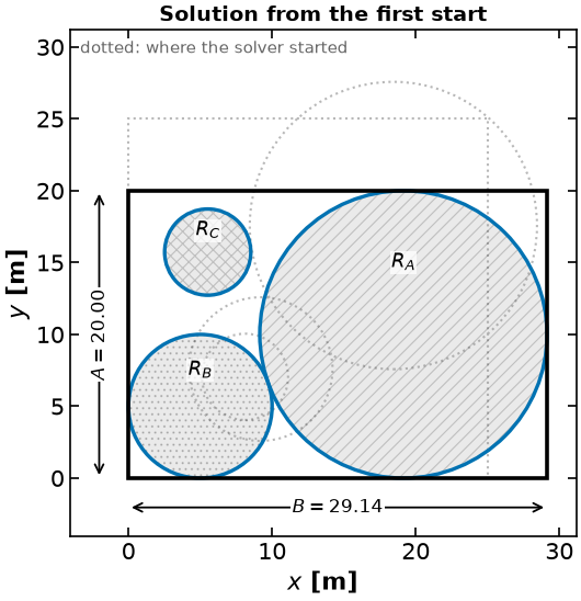
plot_circles(
    extract_circles(model), start=first_start, title="Solution from the first start"
)
plt.show()
Name	Value
box_height 	 19.999999803189603
box_width 	 29.14213541618403
x[A] 	 19.14213551493119
x[B] 	 4.999999951252128
x[C] 	 5.517274811159322
y[A] 	 9.999999901937443
y[B] 	 4.999999953543125
y[C] 	 15.729315741741758
# Print constraints
for c in model.component_data_objects(pyo.Constraint):
    print(
        c.name,
        "\t",
        pyo.value(c.lower),
        "\t",
        pyo.value(c.body),
        "\t",
        pyo.value(c.upper),
    )
left_x_con[A] 10.0 19.14213551493119 None
left_x_con[B] 5.0 4.999999951252128 None
left_x_con[C] 3.0 5.517274811159322 None
left_y_con[A] 10.0 9.999999901937443 None
left_y_con[B] 5.0 4.999999953543125 None
left_y_con[C] 3.0 15.729315741741758 None
right_x_con[A] None 9.87471615587765e-08 0.0
right_x_con[B] None -19.1421354649319 0.0
right_x_con[C] None -20.624860605024708 0.0
right_y_con[A] None 9.874784012708915e-08 0.0
right_y_con[B] None -9.999999849646478 0.0
right_y_con[C] None -1.2706840614478452 0.0
no_overlap_con[A,B] 225.0 224.99999778541928 None
no_overlap_con[A,C] 169.0 218.46188918941948 None
no_overlap_con[B,C] 64.0 115.38579056358046 None
Reinitialize and Resolve
Activity
Reinitialize the model, plot the initial point, resolve, and plot the solution. Is there more than one solution?# Initialize and print the model
# Add your solution here
# Plot initial point
# Add your solution here
# Solve the model
# Add your solution here
# Plot solution
# Add your solution here
The Two Local Solutions, Side by Side
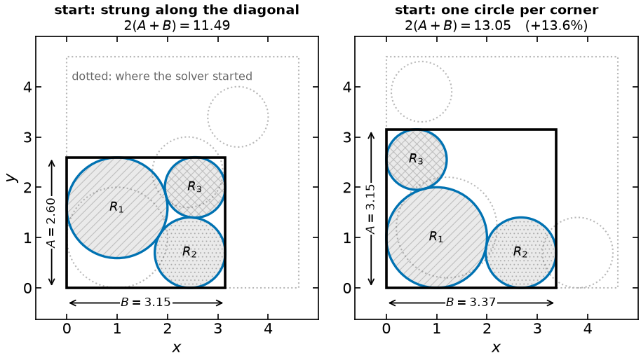
The activity above landed on two different boxes from two different starting arrangements. Let’s do that deliberately, on the instance the lecture handout uses --- , “three circles of different sizes” as Biegler’s Example 4.4 puts it --- and build the figure that appears in the handout.
You can debug the plot without re-solving. Getting three hatched circles, two dimension arrows and a pair of titles to sit where you want them takes a dozen attempts. Each one should cost milliseconds, not a fresh call to Ipopt.
You can archive the answer. Store the extracted numbers next to your paper and you can redraw the figure a year later, on a machine with no solver installed, from the numbers you actually reported.
The plot cell cannot lie about the model. If it only ever sees the extracted results, it cannot quietly recompute something different from what you solved.
In research code, pickle is the quick way to store the extracted results, and that is what we recommend there. Here the archive is committed to this repository, so it is written as JSON instead: a pickle in version control is an unreviewable binary that stops loading the next time a library is upgraded, and nobody can read its diff.
# ---------- SOLVE ----------------------------------------------------------
# Nothing is plotted in this cell. This is the only cell below that needs a
# solver.
#
# THE INSTANCE. Biegler prints no numerical radii -- his Figure 4.4 is a sketch
# -- so R = (1.0, 0.7, 0.6) is ours. It was chosen because it has *two*
# certified local minima that are 13.6% apart in perimeter: far enough that the
# two boxes differ visibly on the page, and the radii are visibly unequal, as
# "three circles of different sizes" requires. Other triples give only one, and
# then the picture below is impossible to draw.
lecture_radii = {"1": 1.0, "2": 0.7, "3": 0.6}

# The loose box every run starts from. Biegler's second bullet on p. 68 is
# "change the initial arrangement of the circles and manually shrink the walls
# of the box", so the starting walls are part of the story and get drawn.
BOX_INIT = 4.6

# Two starting arrangements, both feasible, both describable in words.
starts = {
    "strung along the diagonal": {"1": (1.0, 1.0), "2": (2.4, 2.3), "3": (3.4, 3.4)},
    "one circle per corner": {"1": (1.2, 1.2), "2": (3.8, 0.7), "3": (0.7, 3.9)},
}

# ⚠ R_2 SITS SLIGHTLY OFF THE DIAGONAL ON PURPOSE, and that is a lesson rather
# than bookkeeping. This model is symmetric under swapping the two axes
# (A <-> B and x <-> y together). A start with all three centers exactly on the
# line y = x is a fixed point of that symmetry, and Ipopt walks straight down
# it to the symmetric stationary point: a *square* box, perimeter 14.885, which
# is not a local minimum at all. Measured with Pyomo 6.10.1 + Ipopt: centers
# (1.0, 1.0), (2.3, 2.3), (3.4, 3.4) in a box of 4.6 return 14.885, and the
# same start with the box written as 4.599999999999997 returns 11.488. The
# tie-break is being decided by the last bits of the mantissa. Break the
# symmetry yourself; do not leave it to round-off.


def solve_circle_packing(radii, centers, box_init=BOX_INIT):
    """Build, initialize from a named arrangement, and solve. Returns the model."""
    m = create_circle_model(radii)
    m.box_height = box_init
    m.box_width = box_init
    for i, (x0, y0) in centers.items():
        m.x[i] = x0
        m.y[i] = y0
    status = pyo.SolverFactory("ipopt").solve(m)
    assert pyo.check_optimal_termination(status), (
        f"solve failed: {status.solver.termination_condition}"
    )
    return m


def extract_point(m):
    """Pyomo model -> plain Python. After this, nothing needs the model again."""
    return {
        "A": pyo.value(m.box_height),
        "B": pyo.value(m.box_width),
        "perimeter": pyo.value(m.obj),
        "centers": {i: (pyo.value(m.x[i]), pyo.value(m.y[i])) for i in m.CIRCLES},
    }


points = {
    name: extract_point(solve_circle_packing(lecture_radii, centers))
    for name, centers in starts.items()
}

for name, p in points.items():
    print(
        f"start {name:28s} -> A = {p['A']:.4f} m, B = {p['B']:.4f} m, "
        f"perimeter = {p['perimeter']:.4f} m"
    )

names = list(starts)
penalty = 100.0 * (points[names[1]]["perimeter"] / points[names[0]]["perimeter"] - 1.0)
print(f"the two answers differ by {penalty:.1f}% of the better one")
start strung along the diagonal -> A = 2.5961 m, B = 3.1478 m, perimeter = 11.4880 m
start one circle per corner -> A = 3.1492 m, B = 3.3733 m, perimeter = 13.0450 m
the two answers differ by 13.6% of the better one
# ---------- ARE THEY REALLY LOCAL MINIMA? ----------------------------------
# The caption of the handout figure claims both answers are genuine local
# solutions. That is a claim, so it gets checked.
#
# ⚠ THE OBVIOUS CHECK IS THE WRONG ONE. Perturb the answer, re-solve, see
# whether it comes back: that measures the *basin radius*, not local
# minimality. A genuine local minimum is escaped by any perturbation larger
# than its basin, so run that test with a large perturbation and you will
# conclude, falsely, that this problem has one local solution.
#
# The test used instead is a TRUST-REGION CERTIFICATE. Minimize the objective
# over the feasible set intersected with a ball ||z - z*|| <= delta, from many
# starts inside that ball. If nothing in the ball beats z*, then z* is a local
# minimum out to radius delta. delta = 0.5 is large next to a box of side ~3.
#
# This matters: Ipopt also stops at points that are NOT local minima -- the
# symmetric square box at 14.885 noted above is one, and the certificate
# improves on it immediately.

DELTA = 0.5
N_TRY = 40


def best_in_ball(radii, z_star, delta=DELTA, n_try=N_TRY, seed=17):
    """Smallest perimeter attainable inside ||z - z*|| <= delta and feasible.

    Returns the perimeter at z* itself if nothing in the ball improves on it.
    A smaller value means z* is a point the solver stopped at and nothing more.
    """
    rng = random.Random(seed)  # seeded: an unseeded certificate is not evidence
    circles = list(radii)
    n = 2 + 2 * len(circles)
    m_units = pyo.units.m
    best = z_star["perimeter"]
    opt = pyo.SolverFactory("ipopt")

    for _ in range(n_try):
        # A point uniform in the ball: random direction, radius ~ U(0,1)^(1/n).
        d = [rng.gauss(0.0, 1.0) for _ in range(n)]
        scale = delta * rng.random() ** (1.0 / n) / sum(v * v for v in d) ** 0.5
        d = [v * scale for v in d]

        m = create_circle_model(radii)
        m.box_height = z_star["A"] + d[0]
        m.box_width = z_star["B"] + d[1]
        for k, i in enumerate(circles):
            m.x[i] = z_star["centers"][i][0] + d[2 + 2 * k]
            m.y[i] = z_star["centers"][i][1] + d[3 + 2 * k]

        # The ball itself, as one extra constraint on the same model.
        m.trust_region = pyo.Constraint(
            expr=(m.box_height - z_star["A"] * m_units) ** 2
            + (m.box_width - z_star["B"] * m_units) ** 2
            + sum(
                (m.x[i] - z_star["centers"][i][0] * m_units) ** 2
                + (m.y[i] - z_star["centers"][i][1] * m_units) ** 2
                for i in circles
            )
            <= delta**2 * m_units**2
        )

        status = opt.solve(m)
        if pyo.check_optimal_termination(status):
            best = min(best, pyo.value(m.obj))
    return best


certificate = {}
for name, p in points.items():
    certificate[name] = best_in_ball(lecture_radii, p)
    verdict = "LOCAL MINIMUM" if certificate[name] > p["perimeter"] - 1e-3 else "NOT a minimum"
    print(
        f"{name:28s} perimeter {p['perimeter']:.5f}, best in ball of radius "
        f"{DELTA} = {certificate[name]:.5f}  ->  {verdict}"
    )
strung along the diagonal perimeter 11.48797, best in ball of radius 0.5 = 11.48797 -> LOCAL MINIMUM
one circle per corner perimeter 13.04503, best in ball of radius 0.5 = 13.04503 -> LOCAL MINIMUM
# ---------- ARCHIVE --------------------------------------------------------
# figures/results/packing-local-solutions.json, committed to the repository.
# `source_tag` points at the model cell above, so scripts/check_results_fresh.py
# can tell you when the model has changed and these numbers have not.
# A no-op on Colab, where there is nothing to commit to.

results = {
    "radii": dict(lecture_radii),
    "box_init": BOX_INIT,
    "delta": DELTA,
    "panels": [
        {
            "name": name,
            "start": {i: list(starts[name][i]) for i in starts[name]},
            "A": points[name]["A"],
            "B": points[name]["B"],
            "perimeter": points[name]["perimeter"],
            "centers": {i: list(points[name]["centers"][i]) for i in lecture_radii},
            "best_in_ball": certificate[name],
        }
        for name in starts
    ],
}

helper.save_results(
    "packing-local-solutions",
    results,
    notebook="notebooks/1-dev/NLP.ipynb",
    source_tag="handout:circle-packing-model",
    description="Biegler Example 4.4 with R = (1.0, 0.7, 0.6), solved twice "
    "from two starting arrangements: two local solutions 13.6% apart in "
    "perimeter, each certified by a trust-region check of radius 0.5.",
    solver="Ipopt via Pyomo",
)
[helper] wrote figures/results/packing-local-solutions.json
# The PLOTTING function: it takes the extracted results, not the Pyomo model.
#
# Everything it needs is in `results`, and nothing else -- no model, no solver.
# That is what lets you re-run this one cell as many times as it takes to get
# the labels where you want them.
#
# This cell is tagged `figure:packing-local-solutions`, which makes it the
# single source of the figure the lecture handout prints. See figures/README.md;
# figures/render_from_notebook.py re-runs exactly this cell against the archived
# JSON when the house style changes. That driver binds `helper` for the cell,
# so this cell may use it without importing anything.

from matplotlib.patches import Circle, Rectangle


def plot_packing_local_solutions(results):
    """Two local solutions of the circle-packing NLP, from two starting guesses.

    WHY THIS FIGURE EXISTS. The model above is nonconvex -- the No Overlap
    constraints are -- so the convexity theorem does not apply and

        "the optimum you find depends on where you start."

    This is the evidence for that sentence, and it is Biegler's own second
    bullet on p. 68. Same model, same solver, same tolerances, two starting
    arrangements, two different answers.

    Both are local solutions: neither is refuted by anything local, which is
    the entire content of "no guarantee of a global solution". The certificate
    that says so is computed in the solve cells above and archived alongside
    the coordinates.

    GREYSCALE. The three circles carry three genuinely different hatch families
    -- lines, dots, crosses -- and their own labels, so they are told apart
    without color. The starting arrangement is dotted and unfilled against the
    solid, filled solution: a linestyle contrast, not a color one. The box is
    black in both panels.
    """
    radii = results["radii"]
    panels = results["panels"]
    box0 = results["box_init"]
    circles = list(radii)

    # Hatch literals copied from figures/plots/_house.py, which is NOT on disk
    # on Colab and must not be imported here:
    #   HATCH_CYCLE = ("///", "\\\\\\", "...", "xxx", "|||", "---")
    #   SHADE_ALPHA = 0.18
    # ⚠ HATCH_CYCLE[1], "\\\", is skipped deliberately. Three circles need
    # three textures, and these three spend three different texture FAMILIES,
    # so every pair differs in kind. Restoring [1] puts two of the three in the
    # same family, separated only by the SIGN of the slope -- the most fragile
    # cue here, because the hatch is drawn pale at low alpha inside circles
    # that touch.
    hatches = ("///", "...", "xxx")
    shade_alpha = 0.18
    hatch_colour = plt.rcParams["hatch.color"]
    blue = "#0072B2"  # Okabe-Ito; the solved circles are the only color here
    lim_lo, lim_hi = -0.62, 5.00

    def draw_circles(ax, centers, solution):
        """One arrangement. `solution` toggles solved vs starting guess."""
        for k, i in enumerate(circles):
            x, y = centers[i]
            if solution:
                ax.add_patch(Circle((x, y), radii[i], facecolor="0.55",
                                    alpha=shade_alpha, hatch=hatches[k],
                                    edgecolor=hatch_colour, linewidth=0.0,
                                    zorder=2))
                ax.add_patch(Circle((x, y), radii[i], facecolor="none",
                                    edgecolor=blue, linewidth=2.4, zorder=3))
                ax.annotate("$R_%d$" % (k + 1), xy=(x, y), fontsize=13,
                            ha="center", va="center", zorder=6)
            else:
                ax.add_patch(Circle((x, y), radii[i], facecolor="none",
                                    edgecolor="0.72", linestyle=":",
                                    linewidth=1.5, zorder=1))

    def draw_box(ax, A, B):
        """The enclosing box, with its two dimensions written on it."""
        ax.add_patch(Rectangle((0.0, 0.0), B, A, facecolor="none",
                               edgecolor="black", linewidth=2.6, zorder=4))
        ax.annotate("", xy=(-0.30, 0.0), xytext=(-0.30, A),
                    arrowprops=dict(arrowstyle="<->", color="black", lw=1.3))
        ax.annotate("$A = %.2f$" % A, xy=(-0.30, 0.5 * A), fontsize=12.5,
                    ha="center", va="center", rotation=90,
                    bbox=dict(facecolor="white", edgecolor="none", pad=1.0))
        ax.annotate("", xy=(0.0, -0.30), xytext=(B, -0.30),
                    arrowprops=dict(arrowstyle="<->", color="black", lw=1.3))
        ax.annotate("$B = %.2f$" % B, xy=(0.5 * B, -0.30), fontsize=12.5,
                    ha="center", va="center",
                    bbox=dict(facecolor="white", edgecolor="none", pad=1.0))

    def frame(ax, title):
        """Apply common axes limits, labels, and title to one panel."""
        ax.set_xlim(lim_lo, lim_hi)
        ax.set_ylim(lim_lo, lim_hi)
        ax.set_aspect("equal", adjustable="box")
        ax.set_xlabel("$x$")
        ax.set_title(title, fontsize=13.5)
        ax.set_xticks([0, 1, 2, 3, 4])
        ax.set_yticks([0, 1, 2, 3, 4])

    # ⚠ figsize is set HERE. helper.set_plotting_style() overrides the house
    # default for on-screen readability and render_from_notebook.py does not,
    # so a figure that relied on the default would come out at two different
    # aspect ratios depending on who generated it.
    fig, axes = plt.subplots(1, 2, figsize=(9.6, 5.0))
    axes[0].set_ylabel("$y$")

    penalty = 100.0 * (panels[1]["perimeter"] / panels[0]["perimeter"] - 1.0)
    # ⚠ f-strings, not %-formatting, for these two: scripts/check_greyscale.py
    # blanks any line whose first non-blank character is `%` (it reads it as a
    # Jupyter line magic), so a `% (...)` continuation line makes the whole
    # notebook score "unparseable".
    titles = [
        f"start: {panels[0]['name']}\n$2(A+B) = {panels[0]['perimeter']:.2f}$",
        f"start: {panels[1]['name']}\n$2(A+B) = {panels[1]['perimeter']:.2f}$"
        f"   $(+{penalty:.1f}\\%)$",
    ]

    for ax, panel, title in zip(axes, panels, titles):
        frame(ax, title)
        # The loose box every run starts from: p. 68 is about shrinking these
        # walls, so the walls have to be on the page.
        ax.add_patch(Rectangle((0.0, 0.0), box0, box0, facecolor="none",
                               edgecolor="0.72", linestyle=":", linewidth=1.5,
                               zorder=1))
        draw_circles(ax, panel["start"], solution=False)
        draw_circles(ax, panel["centers"], solution=True)
        draw_box(ax, panel["A"], panel["B"])

    axes[0].annotate("dotted: where the solver started", xy=(0.10, 4.30),
                     fontsize=11.5, ha="left", va="top", color="0.40")

    fig.tight_layout()
    return fig


fig = plot_packing_local_solutions(results)

# Write media/figures/packing-local-solutions.{png,pdf} -- what the lecture
# handout \includegraphics. A no-op on Colab, where there is no repo to write to.
helper.save_figure(fig, "packing-local-solutions")
[helper] wrote media/figures/packing-local-solutions.png and .pdf
Multistart
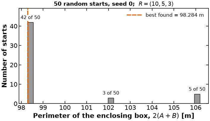
The activity above shows that two starting points can give two different boxes. That raises the obvious question: how many different boxes are there, and how often does the solver find the best one?
A multistart answers that empirically. Solve the same model from many random initial points, collect the objective values, and look at the distribution. Note what this does and does not buy you: it raises confidence that you have found the global solution, but it is never a certificate. Proving global optimality of a nonconvex program requires a global solver, which is a topic for later in the course.
Two practical points before the code:
Seed the random number generator. A histogram built from an unseeded sampler is a different figure every time the notebook runs, and a number you cannot reproduce is a number you cannot defend.
Sample widely enough to matter. The default
spread=10used above draws the centers from a window smaller than the box itself, and essentially every start then lands in the same basin. We widen it below.
def multistart_circle_packing(
    circle_data, n_starts=50, seed=0, spread=40, box_init=40, tee=False
):
    """Solve the circle packing model from many random initial points

    Arguments:
        circle_data: dictionary with keys=circle name and value=radius (float)
        n_starts: number of random initializations (int)
        seed: seed for the random number generator, so the result reproduces
        spread: width of the uniform window the centers are drawn from
        box_init: initial value for both box dimensions
        tee: print solver output

    Returns:
        results: pandas DataFrame, one row per start, with the objective and
            the box dimensions (NaN if that start did not solve)
        arrangements: dict keyed by start, each holding the extracted `start`
            point and the extracted `solution` (None if that start failed).
            This is what lets us go back and LOOK at a chosen solution; the
            DataFrame alone records that the local solutions differ, not what
            any of them looks like.
    """
    # Reproducibility. Reseeding here means this cell gives the same answer no
    # matter which other cells were run first.
    random.seed(seed)

    solver = pyo.SolverFactory("ipopt")

    rows = []
    arrangements = {}
    for k in range(n_starts):
        m = create_circle_model(circle_data)
        initialize_circle_model(
            m, height_init=box_init, width_init=box_init, spread=spread
        )
        # Keep the initial point BEFORE solving -- afterwards it is gone, and
        # for a nonconvex model the initial point is half of what makes an
        # answer reportable.
        # ⚠ Extracting it draws no random numbers, so the sampling sequence,
        # and therefore every number this section prints, is unchanged.
        start_point = extract_circles(m)

        res = solver.solve(m, tee=tee)
        if pyo.check_optimal_termination(res):
            arrangements[k] = {"start": start_point, "solution": extract_circles(m)}
            rows.append(
                {
                    "start": k,
                    "perimeter": pyo.value(m.obj),
                    "A": pyo.value(m.box_height),
                    "B": pyo.value(m.box_width),
                }
            )
        else:
            arrangements[k] = {"start": start_point, "solution": None}
            rows.append(
                {"start": k, "perimeter": float("nan"), "A": float("nan"),
                 "B": float("nan")}
            )

    return pd.DataFrame(rows), arrangements


# The multistart experiment, named ONCE. The archive cell below records these
# four numbers alongside the perimeters, and a literal repeated in two cells is
# a literal that will eventually disagree with itself.
MS_STARTS = 50
MS_SEED = 0
MS_SPREAD = 40
MS_BOX_INIT = 40

ms, ms_points = multistart_circle_packing(
    circle_data,
    n_starts=MS_STARTS,
    seed=MS_SEED,
    spread=MS_SPREAD,
    box_init=MS_BOX_INIT,
)

n_failed = int(ms["perimeter"].isna().sum())
print(f"{len(ms)} starts, {n_failed} failed to converge")
print(f"Best perimeter found: {ms['perimeter'].min():.4f}")
50 starts, 0 failed to converge
Best perimeter found: 98.2843
# How many distinct local solutions did we land on?
counts = (
    ms["perimeter"]
    .round(3)
    .value_counts()
    .rename_axis("perimeter")
    .reset_index(name="number of starts")
    .sort_values("perimeter")
    .reset_index(drop=True)
)
counts["fraction"] = counts["number of starts"] / len(ms)
display(counts)
# ---------- EXTRACT + ARCHIVE ---------------------------------------------
# pandas -> plain Python, then figures/results/packing-multistart-histogram.json,
# committed to the repository. After this cell nothing below touches `ms`, a
# Pyomo model, or a solver: the plotting cell reads `results` and nothing else,
# so the histogram can be redrawn as many times as it takes without paying for
# fifty solves again.
#
# `source_tag` points at the model cell above, so scripts/check_results_fresh.py
# can tell you when the model has changed and these numbers have not. Writing is
# a no-op on Colab, where there is nothing to commit to.
#
# ⚠ WHAT IS ARCHIVED IS THE FIFTY PERIMETERS, NOT THE HISTOGRAM'S BIN HEIGHTS.
# The number of bins is a plotting decision and belongs in the plot cell;
# freezing the bins here would make a *style* change to this figure impossible
# without re-solving, and avoiding exactly that is the archive's only job.
# A start that failed to converge is stored as `null` rather than dropped, so
# the archive still records how many starts were run.

results = {
    "radii": dict(circle_data),
    "n_starts": MS_STARTS,
    "seed": MS_SEED,
    "spread": MS_SPREAD,
    "box_init": MS_BOX_INIT,
    "perimeters": [None if pd.isna(v) else float(v) for v in ms["perimeter"]],
    "best": float(ms["perimeter"].min()),
    # The `counts` table printed above: one row per distinct local solution.
    "spikes": helper.table(counts),
}

helper.save_results(
    "packing-multistart-histogram",
    results,
    notebook="notebooks/1-dev/NLP.ipynb",
    source_tag="handout:circle-packing-model",
    description=(
        "Circle packing on the notebook's instance R = (10, 5, 3): perimeters "
        "from 50 random starts, seed 0, centers drawn uniformly from a window "
        "of width 40. The perimeters fall on three distinct local solutions "
        "rather than a spread."
    ),
    solver="Ipopt via Pyomo",
)
[helper] wrote figures/results/packing-multistart-histogram.json
# The PLOTTING function: it takes the extracted results, not the Pyomo model.
#
# This cell is tagged `figure:packing-multistart-histogram`, which makes it the
# single source of the histogram the lecture handout prints. See
# figures/README.md; figures/render_from_notebook.py re-runs exactly this cell
# against the archived JSON when the house style changes, so there is no second
# copy of the plotting code anywhere. That driver binds `helper` for the cell,
# so this cell may use it without importing anything.


def plot_packing_multistart_histogram(results):
    """Perimeters from many random starts: a few sharp spikes, not a spread.

    WHY THIS FIGURE EXISTS. The two-panel figure earlier in this notebook shows
    that *two* starting arrangements give two different boxes. It cannot show
    how many different boxes there are, or how often the solver finds the best
    one. This does: every start is one sample, and the samples pile up on a
    handful of values because Ipopt converges to a small number of distinct
    local solutions.

    ⚠ THIS IS A LARGER INSTANCE THAN THE TWO-PANEL FIGURE, on purpose --
    R = (10, 5, 3) here against R = (1.0, 0.7, 0.6) there -- so the perimeters
    are around 98 rather than around 11. The two figures are two different
    experiments and must not be read as one; the axis label and the title both
    carry the instance so a reader cannot mistake them.

    THE COUNTS ARE PRINTED, and that is reproducible only because the seed is.
    An unseeded sampler gives a different count every run; with the seed quoted,
    "42 of 50" is a number someone else can obtain. The *best value* is far more
    robust than the count -- it is the same for every seed tried, while the
    split between the spikes is not -- so the best value is drawn as a rule
    across the whole axes and the counts are annotations on the bars.

    GREYSCALE. There is one data series and it is achromatic: grey bars with
    black edges. The only color is the vermillion rule at the best value
    found, which is also DASHED, so it is identified without color.
    """
    perimeters = [p for p in results["perimeters"] if p is not None]
    n_starts = results["n_starts"]
    seed = results["seed"]
    best = results["best"]
    radii = results["radii"]

    # ⚠ figsize is set HERE. helper.set_plotting_style() overrides the house
    # default for on-screen readability and render_from_notebook.py does not,
    # so a figure that relied on the default would come out at two different
    # aspect ratios depending on who generated it.
    fig, ax = plt.subplots(figsize=(7.4, 4.4))

    heights, edges, _ = ax.hist(perimeters, bins=30, color="0.60",
                                edgecolor="black", linewidth=1.0, zorder=2)

    # Okabe-Ito vermillion, from figures/dowling.mplstyle. Plain "red" is not in
    # the palette: it is the color a red-green color-blind reader cannot
    # separate from the black bar edges, and it prints as almost the same grey.
    ax.axvline(best, color="#D55E00", linestyle="--", linewidth=2.4, zorder=3,
               label=f"best found = {best:.3f} m")

    # One annotation per spike, read off the archived counts table rather than
    # typed in: the number of spikes depends on the seed and the sampler, so a
    # hard-coded three would break by drawing the wrong labels rather than by
    # raising an error.
    cols = results["spikes"]["columns"]
    ip, ic = cols.index("perimeter"), cols.index("number of starts")
    rows = results["spikes"]["rows"]

    # ⚠ EACH LABEL IS PLACED OVER ITS BAR, NOT OVER ITS PERIMETER. A spike sits
    # somewhere inside a bin, and a bin here is about 0.26 m wide, so a label
    # centered on the perimeter itself hangs off the side of the bar it belongs
    # to -- and for the leftmost spike, which is the whole point of the figure,
    # off the left edge of the axes entirely. Found by rendering and looking.
    for row in rows:
        k = min(range(len(heights)), key=lambda j: abs(row[ip] - edges[j]))
        k = min(k, len(heights) - 1)
        if row[ip] < edges[k]:
            k = max(k - 1, 0)
        ax.annotate(
            f"{int(row[ic])} of {n_starts}",
            xy=(0.5 * (edges[k] + edges[k + 1]), heights[k]),
            xytext=(0, 5),
            textcoords="offset points",
            ha="center",
            va="bottom",
            fontsize=11.5,
            zorder=4,
            # The label over the tallest bar is crossed by the dashed rule at
            # the best value; a white patch behind the text keeps both legible
            # without moving either off the thing it labels.
            bbox=dict(facecolor="white", edgecolor="none", pad=0.8),
        )

    # Headroom above the tallest bar for its label, and a margin at each end so
    # the outer two labels are not clipped by the frame.
    ax.set_ylim(0, 1.17 * max(heights))
    pad = 0.05 * (edges[-1] - edges[0])
    ax.set_xlim(edges[0] - pad, edges[-1] + pad)

    r_text = ", ".join(f"{radii[i]:g}" for i in radii)
    ax.set_xlabel("Perimeter of the enclosing box, $2(A + B)$ [m]")
    ax.set_ylabel("Number of starts")
    ax.set_title(
        f"{n_starts} random starts, seed {seed};  $R = ({r_text})$", fontsize=13.5
    )
    ax.legend(loc="upper right")

    fig.tight_layout()
    return fig


fig = plot_packing_multistart_histogram(results)

# Write media/figures/packing-multistart-histogram.{png,pdf} -- what the lecture
# handout \includegraphics. A no-op on Colab, where there is no repo to write to.
helper.save_figure(fig, "packing-multistart-histogram")
[helper] wrote media/figures/packing-multistart-histogram.png and .pdf
# Which start gave the best box?
best_start = int(ms["perimeter"].idxmin())
print(f"Best start: #{best_start}")
print(f"  perimeter = {ms.loc[best_start, 'perimeter']:.4f} m")
print(f"  A = {ms.loc[best_start, 'A']:.4f} m, B = {ms.loc[best_start, 'B']:.4f} m")
Best start: #41
  perimeter = 98.2843 m
  A = 20.0000 m, B = 29.1421 m
What Do the Spikes Actually Look Like?
The histogram says there are a handful of distinct local solutions. It does not say what they are. Because the multistart kept every arrangement, we can go back and draw one representative of each spike.
Note how the representatives are chosen: the counts table above is the list of
spikes, so we read them off it rather than typing in three numbers. How many spikes
there are, and how many starts land on each, depends on the seed and on the sampler --
which is the point the discussion below makes. Hard-coding three would quietly break
the moment you change the seed, and it would break by showing you the wrong picture
rather than by raising an error.
# One representative start per spike, chosen programmatically from `counts`.
spikes = ms["perimeter"].round(3)
representatives = [
    {
        "perimeter": p,
        "n_starts": int(n),
        # The first start that landed on this spike. Any member would do; the
        # first is the reproducible choice.
        "start": int(spikes[spikes == p].index[0]),
    }
    for p, n in zip(counts["perimeter"], counts["number of starts"])
]

for r in representatives:
    print(
        f"perimeter {r['perimeter']:.3f} m  <-  {r['n_starts']:2d} of {len(ms)} "
        f"starts, e.g. start #{r['start']}"
    )

# One shared scale across the panels, so the boxes can be compared by eye.
# Without this each panel is fitted to its own contents and the biggest box
# looks the same size as the smallest.
shared_span = max(
    max(ms_points[r["start"]]["solution"]["A"], ms_points[r["start"]]["solution"]["B"])
    for r in representatives
)

fig, axes = plt.subplots(
    1, len(representatives), figsize=(4.6 * len(representatives), 5.2), squeeze=False
)
for ax, r in zip(axes[0], representatives):
    best = " (best found)" if r is representatives[0] else ""
    plot_circles(
        ms_points[r["start"]]["solution"],
        title=(
            f"{r['n_starts']} of {len(ms)} starts{best}\n"
            f"$2(A+B) = {r['perimeter']:.3f}$ m"
        ),
        ax=ax,
        span=shared_span,
    )
    if ax is not axes[0][0]:
        ax.set_ylabel("")
fig.tight_layout()
plt.show()
perimeter 98.284 m  <-  42 of 50 starts, e.g. start #0
perimeter 101.977 m  <-   3 of 50 starts, e.g. start #12
perimeter 106.193 m  <-   5 of 50 starts, e.g. start #20
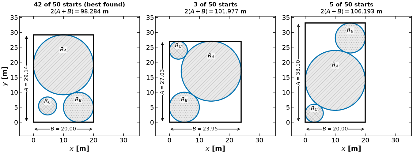
The three packings are genuinely different arrangements, not the same one relabelled: the solver has settled the circles against different walls and into different corners, and each is a point that nothing local can improve on.
⚠ The random initial points are deliberately not drawn underneath here. This
multistart draws its centers from a window of width spread=40, so the starting
arrangement is several times the size of the answer; on a shared scale it would
squeeze all three solutions into a corner and show you nothing. The two-panel figure
earlier in this notebook draws its starting arrangements because they were chosen by
hand, are the same size as the answer, and are part of the story being told.
The histogram has a few sharp spikes, not a smooth spread: Ipopt is converging to a small number of distinct local solutions, and the spikes are those solutions. Most starts find the best one, but a meaningful minority do not.
Three things to take from this:
The best value found is far more reproducible than the fraction that finds it. The best perimeter is the same for every seed we tried; the count is not. If you report a fraction, report the sampler and the seed with it, because the fraction depends on both.
A multistart is evidence, not proof. Fifty starts all agreeing is good evidence that the best value found is global. It is not a certificate, and no number of starts makes it one.
The sampler is part of the experiment. Drawing the centers from a narrow window makes every start look identical and the problem look convex. It is not.
Activity
Change the seed and re-run the multistart. Does the best perimeter change? Does the fraction of starts that find it change? Which of those two would you be willing to put in a report?Take Away Messages
Nonlinear programs may be nonconvex. For nonconvex problems, there often exist many local optima that are not also global optima.
We will learn how to mathematically define convexity and analyze this property.
Initialization is really important in optimization problems with nonlinear objectives or constraints!
There are specialized solvers for linear programs, quadratic programs, and convex programs. In this class, we will focus on more general algorithms for (non)convex nonlinear programs including the algorithms used by the
ipoptsolver.