Portfolio Optimization

Reference: Nocedal and Wright, Numerical Optimization, 2nd ed. (2006), Example 16.1 (Portfolio Optimization), pp. 449--450.

This notebook is adapted from Problem 3 of Problem Set 3 in CBE 20258: Numerical and Statistical Analysis, where it is used to practice statistical analysis. Here we use it as the course’s first convex nonlinear program, and as the foil to the circle packing example: same solver, same course, but the answer is guaranteed to be global.

# This code cell installs packages on Colab

import sys

if "google.colab" in sys.modules:
    !wget "https://raw.githubusercontent.com/ndcbe/optimization/main/notebooks/helper.py"
    import helper

    helper.easy_install()
else:
    sys.path.insert(0, "../")
    import helper
helper.set_plotting_style()

import numpy as np
import pandas as pd
import matplotlib.pyplot as plt
import pyomo.environ as pyo
from pyomo.environ import units as u
from pyomo.util.check_units import assert_units_consistent

The data¶

Historical daily adjusted closing prices for five years (from Yahoo! Finance) are available for the $N = 5$ market indices below. (They are market indices rather than individual stocks, but that does not change the analysis.)

Symbol	Name
DJI	Dow Jones Industrial Average
GSPC	S&P 500
IXIC	NASDAQ Composite
RUT	Russell 2000
VIX	CBOE Volatility Index

df_adj_close = pd.read_csv("https://raw.githubusercontent.com/ndcbe/optimization/main/notebooks/data/Stock_Data.csv")

print(
    f"{len(df_adj_close)} daily closing prices for {len(df_adj_close.columns)} indices"
)
df_adj_close.head()

1259 daily closing prices for 5 indices

Loading...

Step 1. Estimate the model parameters¶

The one-day return rate for index $i$ between days $t$ and $t+1$ is

r_{t,i} = \frac{p_{t+1,i} - p_{t,i}}{p_{t,i}}

(1)

where $p_{t,i}$ is the adjusted closing price. From the matrix of returns $R$ we estimate

$\bar{r}_i$ , the average one-day return of index $i$ , and
$\Sigma_r$ , the covariance matrix of the one-day returns.

Notice that both are estimated from data. Neither was given to us. Hold that thought until the last section.

# One-day return rates. pct_change() computes (p_{t+1} - p_t) / p_t.
R = df_adj_close.pct_change().dropna()

# Average one-day return of each index, rbar_i [1/day]
R_avg = R.mean(axis=0)

# Covariance of the one-day returns, Sigma_ij [1/day^2]
Cov = R.cov()

print(f"{len(R)} one-day returns\n")
print("Average one-day return:")
print(R_avg)

1258 one-day returns

Average one-day return:
DJI     0.000432
GSPC    0.000454
IXIC    0.000674
RUT     0.000440
VIX     0.003718
dtype: float64

print("Covariance matrix:")
display(Cov.round(8))

print("\nCorrelation matrix:")
display(R.corr().round(4))

Covariance matrix:

Loading...


Correlation matrix:

Loading...

Step 2. The Markowitz mean/variance model¶

Given a set of assets whose returns fluctuate, choose what fraction of your money to put in each so that the variance of the portfolio return is as small as possible, subject to achieving at least a required expected return.

Sets. $\mathcal{S}$ --- the assets.

Parameters. $\bar{r}_i$ , the expected one-day return of asset $i \in \mathcal{S}$ ; $\Sigma_r$ , the covariance matrix of the one-day returns; $\rho$ , the required expected return of the portfolio.

Variables. $x_i$ , the fraction of funds placed in asset $i$ .

\begin{align} \min_{x} \quad & z := x^T \Sigma_r x && \text{variance of the portfolio return} \\ \text{s.t.} \quad & \bar{r}^T x \geq \rho && \text{achieve the required return} \\ & \sum_{i \in \mathcal{S}} x_i = 1 && \text{invest all of it} \\ & x_i \geq 0 \quad \forall i \in \mathcal{S} && \text{no short selling} \end{align}

(2)

The objective is quadratic and every constraint is linear, so this is a quadratic program. Because $\Sigma_r$ is a covariance matrix it is symmetric positive semidefinite, the Hessian of the objective is $2 \Sigma_r$ , and the feasible set is an intersection of half-spaces with a hyperplane. The problem is therefore convex: every local minimum is a global minimum.

Units. The decision variables are fractions of the portfolio, so they are dimensionless; the mean returns are per-day rates and the covariance is per-day-squared. The builder below declares all three with units= and then calls assert_units_consistent, so no model can leave the function without having been checked. Declaring units and never checking them is worse than not declaring them --- it looks verified.

def create_portfolio_model(rho, r_avg, cov):
    """Create the Markowitz mean/variance portfolio model in Pyomo

    Arguments:
        rho: required expected return of the portfolio (float)
        r_avg: average one-day return of each asset (pandas Series)
        cov: covariance matrix of the one-day returns (pandas DataFrame)

    Returns:
        m: Pyomo concrete model
    """

    m = pyo.ConcreteModel()

    # Set of assets, S in the notes
    m.ASSETS = pyo.Set(initialize=list(r_avg.index))

    # Required expected return of the portfolio, rho [1/day]
    m.rho = pyo.Param(initialize=rho, mutable=True, units=1 / u.day)

    # Expected one-day return of asset i, rbar_i [1/day]
    m.r_avg = pyo.Param(m.ASSETS, initialize=r_avg.to_dict(), units=1 / u.day)

    # Covariance of the one-day returns, Sigma_ij [1/day^2]
    m.cov = pyo.Param(
        m.ASSETS,
        m.ASSETS,
        initialize={(i, j): cov.loc[i, j] for i in m.ASSETS for j in m.ASSETS},
        units=1 / u.day**2,
    )

    # Funds placed in asset i, x_i [dimensionless]. No short selling, so x_i >= 0.
    m.x = pyo.Var(
        m.ASSETS, domain=pyo.NonNegativeReals, initialize=0.0, units=u.dimensionless
    )

    # Minimize the variance of the portfolio return [1/day^2]
    @m.Objective(sense=pyo.minimize)
    def OBJ(b):
        return sum(b.x[i] * b.cov[i, j] * b.x[j] for i in b.ASSETS for j in b.ASSETS)

    # Achieve at least the required expected return [1/day]
    @m.Constraint()
    def required_return(b):
        return sum(b.r_avg[i] * b.x[i] for i in b.ASSETS) >= b.rho

    # Invest all of it [dimensionless]
    @m.Constraint()
    def budget(b):
        return sum(b.x[i] for i in b.ASSETS) == 1

    # Raises UnitsError if any constraint or the objective is inconsistent
    assert_units_consistent(m)

    return m

Step 3. Solve¶

Solve for $\rho = 0.08\%$ per day and report the optimal allocation of funds and the standard deviation of the portfolio return.

rho = 0.0008
m = create_portfolio_model(rho, R_avg, Cov)

solver = pyo.SolverFactory("ipopt")
results = solver.solve(m)
assert pyo.check_optimal_termination(results), (
    f"Solve failed: status={results.solver.status}, "
    f"termination={results.solver.termination_condition}"
)

std_dev = np.sqrt(pyo.value(m.OBJ))
print(f"Standard deviation of the return rate = {std_dev:.6f} per day\n")

print("Optimal allocation of funds:")
for i in m.ASSETS:
    print(f"  {i:>5s}  {pyo.value(m.x[i]) * 100:6.2f}%")

print(
    f"\nExpected return = {sum(pyo.value(m.r_avg[i] * m.x[i]) for i in m.ASSETS):.6f} per day"
)

Standard deviation of the return rate = 0.004580 per day

Optimal allocation of funds:
    DJI   30.55%
   GSPC   18.54%
   IXIC   42.92%
    RUT    0.06%
    VIX    7.93%

Expected return = 0.000800 per day

Activity

Every constraint in this model is linear and the objective is quadratic. Where, then, is the nonlinearity, and what does it cost you?

Step 4. Sweep $\rho$ --- the efficient frontier¶

Increasing the required return $\rho$ forces the optimizer to accept more risk. Tracing the trade-off gives the efficient frontier: the price of return, paid in variance.

rho_vals = np.arange(0.0005, 0.0038, 0.0001)

rows = []
for rho in rho_vals:
    # Build a fresh model at each rho. Reusing one model warm-starts Ipopt from
    # the previous solution, which shifts the last digit of the answer.
    m_rho = create_portfolio_model(rho, R_avg, Cov)
    results = solver.solve(m_rho)
    assert pyo.check_optimal_termination(results), f"Solve failed at rho = {rho}"
    rows.append(
        [rho, np.sqrt(pyo.value(m_rho.OBJ))]
        + [pyo.value(m_rho.x[i]) for i in m_rho.ASSETS]
    )

frontier = pd.DataFrame(rows, columns=["rho", "std_dev"] + list(m_rho.ASSETS))
display(frontier.round(6))

Loading...

fig, ax = plt.subplots(figsize=(6, 4))
ax.plot(frontier["std_dev"], frontier["rho"], "o-")
ax.set_xlabel("Standard deviation of the return rate [per day]")
ax.set_ylabel("Required return $\\rho$ [per day]")
ax.set_title("Efficient frontier")
ax.grid(True)
plt.tight_layout()
plt.show()

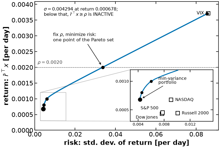
The required return is not always binding¶

Read the first row of the sweep. The minimum-variance portfolio already returns more per day than $\rho = 0.0005$ demands, so the return constraint is inactive at that $\rho$ : deleting it would not change the answer. An inequality constraint you wrote down need not cost you a degree of freedom.

This also explains a discrepancy worth knowing about. The problem set this example comes from states the return requirement as an inequality, $\bar{r}^T x \geq \rho$ , but its solution code writes == rho. At $\rho = 0.0008$ the two agree, because the constraint is active. Below the minimum-variance return they do not.

# The minimum-variance portfolio: drop the return requirement entirely.
m_min = create_portfolio_model(0.0, R_avg, Cov)
m_min.required_return.deactivate()
results = solver.solve(m_min)
assert pyo.check_optimal_termination(results), "Solve failed"

min_var_sd = np.sqrt(pyo.value(m_min.OBJ))
min_var_return = sum(pyo.value(m_min.r_avg[i] * m_min.x[i]) for i in m_min.ASSETS)

print(
    f"Minimum-variance portfolio: sd = {min_var_sd:.6f}, return = {min_var_return:.6f} per day"
)
print(
    f"So the constraint rbar^T x >= 0.0005 is inactive ({min_var_return:.6f} > 0.0005)."
)

Minimum-variance portfolio: sd = 0.004297, return = 0.000679 per day
So the constraint rbar^T x >= 0.0005 is inactive (0.000679 > 0.0005).

Where the data came from¶

Neither $\bar{r}$ nor $\Sigma_r$ was given to us: both were estimated from historical daily returns. They are therefore random variables in their own right, and we can say how uncertain they are. The standard error of a mean estimated from $n$ observations is $s_i / \sqrt{n}$ .

se = R.std(axis=0) / np.sqrt(len(R))

summary = pd.DataFrame({"rbar": R_avg, "standard error": se, "ratio": R_avg / se})
display(summary.round(6))

Loading...

Every mean return in the model is known only to within roughly a factor of two of itself. The constraint $\bar{r}^T x \geq \rho$ has coefficients that wobble by half their own size --- and we then solved to six significant figures.

Optimizing a model to a precision its data cannot support is the most common way to be confidently wrong.

Two caveats on the table above, both of which matter:

$s_i / \sqrt{n}$ assumes the daily returns are independent and identically distributed. Financial returns are neither.
The standard error is itself an estimate.

Quantifying and then optimizing under this kind of uncertainty is what the stochastic programming lectures are for.

Take away messages¶

A quadratic objective with linear constraints is a quadratic program. If the Hessian is positive semidefinite the problem is convex, and a local solution is a global solution.
Contrast with circle packing: same solver, but there the answer depends on where you start, and here it does not.
An inequality constraint that is inactive at the solution costs you nothing. Whether it is active is a property of the solution, not of the model you wrote down.
Parameters estimated from data carry uncertainty. Report it, or at least know it.

The data¶

Step 1. Estimate the model parameters¶

Step 2. The Markowitz mean/variance model¶

Step 3. Solve¶

Step 4. Sweep ρ\rhoρ --- the efficient frontier¶

The required return is not always binding¶

Where the data came from¶

Take away messages¶

Step 4. Sweep $\rho$ --- the efficient frontier¶