Adapted, with thanks, from work by the late Jeffrey Kantor.
This notebook is adapted from notebook 5.1, Milk pooling and blending, in the companion notebook collection for M. Postek, A. Zocca, J. Gromicho and J. Kantor, Hands-On Mathematical Optimization with Python (Cambridge University Press, 2025). Jeff Kantor was a colleague in this department; the example, the data and the framing of the three options are his.
The underlying problem is the canonical pooling benchmark of C. A. Haverly, “Studies of the behavior of recursion for the pooling problem,” ACM SIGMAP Bulletin 25 (1978), 19--28.
MIT License

Copyright (c) 2022 Jeffrey Kantor

Permission is hereby granted, free of charge, to any person obtaining a copy
of this software and associated documentation files (the "Software"), to deal
in the Software without restriction, including without limitation the rights
to use, copy, modify, merge, publish, distribute, sublicense, and/or sell
copies of the Software, and to permit persons to whom the Software is
furnished to do so, subject to the following conditions:

The above copyright notice and this permission notice shall be included in all
copies or substantial portions of the Software.

THE SOFTWARE IS PROVIDED "AS IS", WITHOUT WARRANTY OF ANY KIND, EXPRESS OR
IMPLIED, INCLUDING BUT NOT LIMITED TO THE WARRANTIES OF MERCHANTABILITY,
FITNESS FOR A PARTICULAR PURPOSE AND NONINFRINGEMENT. IN NO EVENT SHALL THE
AUTHORS OR COPYRIGHT HOLDERS BE LIABLE FOR ANY CLAIM, DAMAGES OR OTHER
LIABILITY, WHETHER IN AN ACTION OF CONTRACT, TORT OR OTHERWISE, ARISING FROM,
OUT OF OR IN CONNECTION WITH THE SOFTWARE OR THE USE OR OTHER DEALINGS IN THE
SOFTWARE.
What is different here. The models are rewritten with named pyo.Set and pyo.Param components so that the Pyomo code reads as the set-notation model in the lecture notes, the solver is ipopt throughout rather than appsi_highs, all three options are built by a single function rather than two, and the convex (McCormick) relaxation is left to the global optimization lecture. The notebook is organized on the course’s five-step procedure, with the three options carried through every step in parallel. Two typographical errors in the source notebook’s mathematics are corrected: its blending constraints are printed with the summation running over the cross product inside a constraint that is already quantified for all , and the sum must run over alone. Its Pyomo code is correct as written.
# This code cell installs packages on Colab

import sys

if "google.colab" in sys.modules:
    !wget "https://raw.githubusercontent.com/ndcbe/optimization/main/notebooks/helper.py"
    import helper

    helper.easy_install()
else:
    sys.path.insert(0, "../")
    import helper
helper.set_plotting_style()

# `helper` also provides the extract / archive / figure plumbing used below.
import numpy as np
import pandas as pd
import matplotlib.pyplot as plt
import pyomo.environ as pyo
from pyomo.environ import units as u
from pyomo.util.check_units import assert_units_consistent

# The source data is scale-free: milk is measured in "units" and priced per unit.
# Pyomo's unit library has neither, so declare both. Fat content stays
# dimensionless -- it is a mass fraction, kg of fat per kg of milk.
u.load_definitions_from_strings(["USD = [currency]", "milk = [milk]"])
Step 0: Problem statement
A bulk distributor supplies custom milk blends to several customers. Each customer specifies a minimum fat content, pays a fixed price per unit, and will buy no more than a stated maximum. The distributor sources raw milk from local farms, each producing milk of known fat content at a known cost.
The distributor has found cheaper raw milk at some remote farms. But it owns only one truck with a single tank for the remote route, so milk from the remote farms must be mixed in that tank before transport. That creates a pool of uniform composition, which is then blended with local milk to meet each customer’s requirement.
Three options:
Business as usual --- local farms only.
Buy a second truck --- keep each remote farm’s milk separate, so everything blends freely.
Pool the remote farms --- one truck, one tank, one composition.
Options 1 and 2 are linear programs. Option 3 is not, and that is the point of the example.
The rest of the notebook follows the course’s five-step procedure --- mathematical model, degree of freedom analysis, Pyomo implementation, analysis of the results --- and works all three options through each step side by side.
customers = pd.DataFrame(
    {
        "Customer 1": {"min_fat": 0.045, "price": 52.0, "demand": 6000.0},
        "Customer 2": {"min_fat": 0.030, "price": 48.0, "demand": 2500.0},
        "Customer 3": {"min_fat": 0.040, "price": 50.0, "demand": 4000.0},
    }
).T

suppliers = pd.DataFrame(
    {
        "Farm A": {"fat": 0.045, "cost": 45.0, "location": "local"},
        "Farm B": {"fat": 0.030, "cost": 42.0, "location": "local"},
        "Farm C": {"fat": 0.033, "cost": 37.0, "location": "remote"},
        "Farm D": {"fat": 0.050, "cost": 45.0, "location": "remote"},
    },
).T

# Farm and customer names
local_farms = suppliers.index[suppliers["location"] == "local"].tolist()
remote_farms = suppliers.index[suppliers["location"] == "remote"].tolist()
all_farms = local_farms + remote_farms
customer_names = customers.index.tolist()

# Problem data as plain dictionaries, keyed by farm or customer name

# Fat fraction of the milk from farm s, phi_s [dimensionless]
fat = suppliers["fat"].astype(float).to_dict()

# Purchase cost per unit from farm s, kappa_s [USD/milk]
cost = suppliers["cost"].astype(float).to_dict()

# Price paid per unit by customer k, pi_k [USD/milk]
price = customers["price"].astype(float).to_dict()

# Maximum demand of customer k, d_k [milk]
demand = customers["demand"].astype(float).to_dict()

# Minimum fat fraction customer k accepts, phi_min_k [dimensionless]
min_fat = customers["min_fat"].astype(float).to_dict()

print("Customers")
display(customers)

print("Suppliers")
display(suppliers)
Customers
Suppliers
Step 1: Mathematical model
It is tempting to write three models. Do not. All three options are the same model under different restrictions, and only one question changes between them:
Which farms can we buy from, and which of those must share the single tanker?
| Option | freely blended, | pooled, | model class |
|---|---|---|---|
| 1. Business as usual | local farms | empty | LP |
| 2. Buy a second truck | all farms | empty | LP |
| 3. Pool the remote farms | local farms | remote farms | bilinear NLP |
Sets. , the farms whose milk blends freely; , the farms that must share one tanker; , every farm we buy from; , the customers.
Parameters. , the fat fraction of farm ’s milk [dimensionless]; , its cost per unit [USD/milk]; , the price customer pays [USD/milk]; , its maximum demand [milk]; , the minimum fat fraction it accepts [dimensionless].
The three subsections below write out each option in that notation. Read them together: Options 1 and 2 are the same equations over different farm sets, and Option 3 is those equations with a pool bolted on.
Option 1: business as usual
Only the local farms, and nothing is pooled: is the local farms and . The one decision variable is , the amount of milk from farm blended into the delivery to customer [milk].
The blend quality constraint is the only one worth pausing on. It says the fat delivered to customer is at least the fraction of the milk delivered to customer , which is a linear statement even though “average fat fraction” is a ratio: multiplying through by the denominator clears it. Every term is linear, so this is a linear program.
Option 2: a second truck
A second truck means each remote farm’s milk travels in its own tank, so it blends freely exactly like the local milk. Nothing is pooled, so is still empty --- the remote farms simply move into :
The equations are the ones written for Option 1, unchanged. It is still a linear program, and it is a relaxation of Option 3: everything Option 3 can do, Option 2 can do too, by sending the same milk down four separate tanks instead of one. So Option 2’s profit is an upper bound on Option 3’s.
Option 3: pool the remote farms
Only one truck is available for the remote route, so purchases from the remote farms are combined into a single pool of uniform composition, transported, and then blended with local milk. Now is the local farms and the remote ones.
This is the -parameterization of the pooling problem: the pool composition is itself a decision variable, .
Variables. , local milk shipped from to customer ; , milk bought from remote farm ; , pooled milk delivered to customer ; and , the fat fraction of the pool.
Every variable is nonnegative, , and is bounded below and above by the smallest and largest fat fractions among the remote farms --- a pool cannot be richer than its richest input.
The pool fat balance can be written either as , as above and as the Pyomo code below does, or as . The two agree on the feasible set, because the pool balance constraint immediately above forces .
The last two constraints contain bilinear terms: a product of the composition variable with a flow variable. A bilinear term is smooth and differentiable everywhere, and irreducibly nonconvex. Unlike an absolute value, no change of variables removes it.
This is the model, and Options 1 and 2 are inside it. Set : there is no tanker, so , and are never declared, the pool balance and pool fat balance disappear, the term in the blend quality constraint is zero, and what is left is exactly the linear program of Option 1. The nonconvexity appears exactly when is non-empty. The model class in the table above is a consequence of the restriction, not an independent choice.
Step 2: Degree of freedom analysis
Before writing any code, count. Following the recipe in Pyomo Nuts and Bolts:
degrees of freedom = number of variables number of equality constraints
inequality constraints and variable bounds are counted separately, and do not subtract. An inequality you wrote down need not cost you a degree of freedom: it costs one only if it is active at the solution, and which ones those are is not known until we solve.
more equality constraints than variables would mean the model is over-specified and there is nothing left to optimize. That is the failure this count is looking for.
With three customers and local farms, remote farms:
Option 1: business as usual
is the two local farms, , .
| count | ||
|---|---|---|
| variables | ||
| equality constraints | 0 | |
| degrees of freedom | ||
| inequality constraints | 3 demand, 3 blend quality | |
| bounds | 6 |
Six degrees of freedom, no equality constraints: nothing is over-specified, and the optimum is determined entirely by which inequalities become active.
Option 2: a second truck
Identical in structure; only is bigger --- all four farms.
| count | ||
|---|---|---|
| variables | ||
| equality constraints | 0 | |
| degrees of freedom | ||
| inequality constraints | 6 | 3 demand, 3 blend quality |
| bounds | 12 |
The number of constraints did not change; only the number of ways to satisfy them. That is what “a second truck” buys.
Option 3: pool the remote farms
| count | ||
|---|---|---|
| variables | , , , | |
| equality constraints | 2 | pool balance, pool fat balance |
| degrees of freedom | ||
| inequality constraints | 6 | 3 demand, 3 blend quality |
| bounds | 12 | ; ; |
Option 3 has the same number of variables as Option 2 and two fewer degrees of freedom. That is the whole economics of the problem in one line: the pool is a restriction, and the two equality constraints are how it bites.
Two cautions about what this count does not tell you.
It is blind to nonconvexity. The two bilinear terms live in the pool fat balance and the blend quality constraints, and a degree of freedom count is identical whether a constraint is linear or not. Options 2 and 3 differ by two equalities in this table and by the entire difficulty of the problem in practice.
Ten degrees of freedom does not mean ten free choices at the optimum. Six inequalities and twelve bounds are waiting, and the active ones are what pins the solution down.
Activity
The three tables above were written by hand. Step 3 prints the same four numbers straight out of Pyomo. Predict them before you run it --- and if a number disagrees, trust neither until you know which one is wrong.Step 3: Pyomo implementation
One function, create_milk_model(local, pooled), and the two arguments are the two halves of the question from Step 1:
| Option | call |
|---|---|
| 1. Business as usual | create_milk_model(local_farms, []) |
| 2. Buy a second truck | create_milk_model(all_farms, []) |
| 3. Pool the remote farms | create_milk_model(local_farms, remote_farms) |
There is no second builder. Farms in local blend freely; farms in pooled share one tanker. If pooled is empty the pool variables are never declared and Pyomo is handed a linear program --- the code reduces the same way the mathematics did in Step 1.
Units. Milk here is measured in generic units, so the notebook declares a milk
unit and a USD currency and hangs them on every Param and Var. Fat content stays
dimensionless, because it is a mass fraction. The builder ends with
assert_units_consistent, which is the part that earns the declaration: it is what
would catch a price or a cost mixed into a constraint that balances amounts of
milk. It cannot catch everything: fat content is dimensionless, so a fat balance
and a milk balance carry the same units.
def create_milk_model(local, pooled):
    """Create the milk blending/pooling model in Pyomo

    One model covers all three options. The only thing that changes is which
    farms are reachable, and which of them must share the single tanker:

        Option 1  local=local_farms, pooled=[]            business as usual
        Option 2  local=all_farms,   pooled=[]            a second truck
        Option 3  local=local_farms, pooled=remote_farms  one truck, one pool

    Farms in `local` blend freely: their milk reaches each customer as its own
    stream z_{l,k}. Farms in `pooled` share one tanker, so their milk is first
    mixed into a single stream of composition p and only then blended. If
    `pooled` is empty there is no tanker, the pool variables are never
    declared, and every remaining term is linear -- the model is an LP.

    Arguments:
        local: list of farm names whose milk blends freely
        pooled: list of farm names whose milk must share one tanker

    Returns:
        m: Pyomo concrete model
    """
    m = pyo.ConcreteModel("Milk blending and pooling")

    # Freely blended farms, L in the notes
    m.L = pyo.Set(initialize=local)

    # Pooled farms, R in the notes. Empty for Options 1 and 2.
    m.R = pyo.Set(initialize=pooled)

    # All farms sourced from, L union R
    m.S = pyo.Set(initialize=list(local) + list(pooled))

    # Customers, K in the notes
    m.K = pyo.Set(initialize=customer_names)

    # Fat fraction of the milk from farm s, phi_s [dimensionless]
    m.fat = pyo.Param(m.S, initialize={s: fat[s] for s in m.S})

    # Purchase cost per unit from farm s, kappa_s [USD/milk]
    m.cost = pyo.Param(m.S, initialize={s: cost[s] for s in m.S}, units=u.USD / u.milk)

    # Price paid per unit by customer k, pi_k [USD/milk]
    m.price = pyo.Param(m.K, initialize=price, units=u.USD / u.milk)

    # Maximum demand of customer k, d_k [milk]
    m.demand = pyo.Param(m.K, initialize=demand, units=u.milk)

    # Minimum fat fraction customer k accepts, phi_min_k [dimensionless]
    m.min_fat = pyo.Param(m.K, initialize=min_fat)

    # Freely blended milk from farm l to customer k, z_{l,k} [milk]
    m.z = pyo.Var(m.L, m.K, domain=pyo.NonNegativeReals, units=u.milk)

    # THE POOL. Declared only when there is one.
    if len(m.R) > 0:
        # Milk bought from pooled farm r, x_r [milk]
        m.x = pyo.Var(m.R, domain=pyo.NonNegativeReals, units=u.milk)

        # Pooled milk delivered to customer k, y_k [milk]
        m.y = pyo.Var(m.K, bounds=lambda b, k: (0, b.demand[k]), units=u.milk)

        # Fat fraction of the pool, p [dimensionless]. A pool cannot be richer
        # than its richest input, nor leaner than its leanest.
        m.p = pyo.Var(bounds=(min(fat[r] for r in pooled), max(fat[r] for r in pooled)))

        # What is bought from the pooled farms is what leaves the pool [milk]
        @m.Constraint()
        def pool_balance(b):
            return sum(b.x[r] for r in b.R) == sum(b.y[k] for k in b.K)

        # Fat into the pool equals fat out. BILINEAR. [milk]
        #
        # The right-hand side is written p * sum_R x_r, while the written model
        # states it as p * sum_K y_k. Those are the same quantity ONLY because
        # pool_balance above forces the two sums to be equal -- what goes into
        # the pool is what leaves it. Delete that constraint and these two
        # forms stop agreeing.
        @m.Constraint()
        def pool_quality(b):
            return sum(b.fat[r] * b.x[r] for r in b.R) == b.p * sum(b.x[r] for r in b.R)

    # Helper expressions, written so the constraints below read the same way
    # whether or not a pool exists.
    def pooled_milk(b, k):
        return b.y[k] if len(b.R) > 0 else 0.0

    def pooled_fat(b, k):
        return b.p * b.y[k] if len(b.R) > 0 else 0.0

    # Maximize profit [USD]
    @m.Objective(sense=pyo.maximize)
    def profit(b):
        revenue_and_cost_local = sum(
            (b.price[k] - b.cost[l]) * b.z[l, k] for l in b.L for k in b.K
        )
        if len(b.R) == 0:
            return revenue_and_cost_local
        return (
            revenue_and_cost_local
            + sum(b.price[k] * b.y[k] for k in b.K)
            - sum(b.cost[r] * b.x[r] for r in b.R)
        )

    # Deliveries cannot exceed each customer's demand [milk]
    @m.Constraint(m.K)
    def demand_limit(b, k):
        return sum(b.z[l, k] for l in b.L) + pooled_milk(b, k) <= b.demand[k]

    # Each delivery meets its fat spec. BILINEAR when a pool exists. [milk]
    @m.Constraint(m.K)
    def blend_quality(b, k):
        fat_delivered = pooled_fat(b, k) + sum(b.fat[l] * b.z[l, k] for l in b.L)
        milk_delivered = sum(b.z[l, k] for l in b.L) + pooled_milk(b, k)
        return fat_delivered >= b.min_fat[k] * milk_delivered

    # Raises UnitsError if any constraint or the objective is inconsistent
    assert_units_consistent(m)

    return m
def model_size(m, label):
"""Count what Pyomo actually built, to check the analysis in Step 2.
Arguments:
m: a Pyomo concrete model
label: name to print above the counts
"""
constraints = list(m.component_data_objects(pyo.Constraint, active=True))
n_var = sum(1 for _ in m.component_data_objects(pyo.Var, active=True))
n_eq = sum(1 for c in constraints if c.equality)
n_ineq = len(constraints) - n_eq
print(label)
print(f" variables {n_var:3d}")
print(f" equality constraints {n_eq:3d}")
print(f" inequality constraints {n_ineq:3d}")
print(f" degrees of freedom {n_var - n_eq:3d}\n")Option 1: business as usual
m1 = create_milk_model(local_farms, [])
model_size(m1, "Option 1: local farms only")
Option 1: local farms only
variables 6
equality constraints 0
inequality constraints 6
degrees of freedom 6
Option 2: a second truck
m2 = create_milk_model(all_farms, [])
model_size(m2, "Option 2: all farms, one truck each")
Option 2: all farms, one truck each
variables 12
equality constraints 0
inequality constraints 6
degrees of freedom 12
Option 3: pool the remote farms
The pool block is the only part of the builder that Options 1 and 2 skip. Its two equality constraints are exactly the two that Step 2 counted.
m3 = create_milk_model(local_farms, remote_farms)
model_size(m3, "Option 3: remote farms pooled")
Option 3: remote farms pooled
variables 12
equality constraints 2
inequality constraints 6
degrees of freedom 10
Step 4: Analyze results
One model means one report function. The pool rows appear only when there is a pool.
Ipopt solves all three. Options 1 and 2 are linear programs and an interior point method is not the fastest way to solve them, but using one solver throughout keeps the comparison clean --- any difference between the three answers is a difference between the three models, not between two pieces of software.
solver = pyo.SolverFactory("ipopt")


def solve_and_report(m, title, opt=None):
    """Solve one option and print the supplier and customer tables.

    Arguments:
        m: a Pyomo concrete model from create_milk_model
        title: heading printed above the tables
        opt: solver to use; defaults to Ipopt with no options set

    Returns:
        the optimal profit
    """
    opt = solver if opt is None else opt
    results = opt.solve(m)
    assert pyo.check_optimal_termination(results), f"Solve failed for {title}"

    pooled = len(m.R) > 0

    print(f"{title}")
    if pooled:
        print(f"  pool composition p = {pyo.value(m.p):6.4f}")
    print(f"  profit             = {pyo.value(m.profit):,.2f}\n")

    # One row per farm: what its milk cost, and where it went.
    rows = []
    for s in m.S:
        row = {"fat": pyo.value(m.fat[s]), "cost": pyo.value(m.cost[s])}
        for k in m.K:
            row[k] = pyo.value(m.z[s, k]) if s in m.L else 0.0
        if pooled:
            row["Pool"] = pyo.value(m.x[s]) if s in m.R else 0.0
        rows.append(row)
    print("  Supplier report")
    display(pd.DataFrame(rows, index=list(m.S)).round(4))

    # One row per customer: what was delivered, and at what fat fraction.
    rows = []
    for k in m.K:
        row = {"min_fat": pyo.value(m.min_fat[k]), "demand": pyo.value(m.demand[k])}
        for l in m.L:
            row[l] = pyo.value(m.z[l, k])
        total = sum(pyo.value(m.z[l, k]) for l in m.L)
        fat_out = sum(pyo.value(m.z[l, k]) * pyo.value(m.fat[l]) for l in m.L)
        if pooled:
            row["Pool"] = pyo.value(m.y[k])
            total += pyo.value(m.y[k])
            fat_out += pyo.value(m.y[k]) * pyo.value(m.p)
        row["Total"] = total
        row["fat delivered"] = fat_out / total if total > 0 else np.nan
        rows.append(row)
    print("  Customer report")
    display(pd.DataFrame(rows, index=list(m.K)).round(4))

    return pyo.value(m.profit)
Option 1: business as usual
profit_1 = solve_and_report(m1, "Option 1, local farms only")Option 1, local farms only
profit = 81,000.00
Supplier report
Customer report
Both local farms are used, and both blend constraints bind. This is the baseline the other two options have to beat, and there is nothing subtle about it: the LP has a unique optimum and any solver finds it.
Option 2: a second truck
profit_2 = solve_and_report(m2, "Option 2, all farms, one truck each")Option 2, all farms, one truck each
profit = 122,441.18
Supplier report
Customer report
Sourcing from the remote farms is worth a great deal --- but Option 2 needs a second truck to keep the two remote supplies separated in transit. Note also that the local farms are displaced entirely, and that Customer 2 is delivered milk richer than it requires. That is product giveaway: the optimizer hands over quality because the alternative costs more.
Option 3: pool the remote farms
This is the only one of the three that is hard, and the rest of this step is about why.
nlp_solver = pyo.SolverFactory("ipopt")

nlp_solver.options["bound_frac"] = 0.01
profit_3 = solve_and_report(m3, "Option 3, pooled, bound_frac = 0.01", nlp_solver)
Option 3, pooled, bound_frac = 0.01
pool composition p = 0.0330
profit = 102,833.33
Supplier report
Customer report
Solve it twice.
bound_frac is an Ipopt option that controls only how far inside its bounds the solver places the initial point. It changes nothing about the model. Solve the same model with two values of it.
nlp_solver.options["bound_frac"] = 0.5
m3_alt = create_milk_model(local_farms, remote_farms)
profit_3_alt = solve_and_report(
    m3_alt, "Option 3, pooled, bound_frac = 0.5", nlp_solver
)
Option 3, pooled, bound_frac = 0.5
pool composition p = 0.0450
profit = 101,392.16
Supplier report
Customer report
Activity
Same model, same solver, same tolerances. One option changed, and it only affects where the solver starts. Which of the two answers is right, and how would you know?Why: fix and look.
If is held fixed, every remaining constraint is linear and the problem is an LP. Sweeping over its range and solving the LP at each value shows the profit as a function of the pool composition. It has three local maxima.
It is tempting to say that Ipopt converges to whichever one it starts nearest. That is false, and this model is the counterexample: reading Ipopt’s pushed-in initial point back with max_iter = 0, bound_frac = 0.5 starts at 0.0415 and bound_frac = 0.4 starts it at 0.0398 --- essentially on the local maximum near 0.040 --- and both converge to 0.045. The reason is the teachable part: bound_frac pushes every variable off its bounds, so the twelve-vector the barrier method actually starts from is nowhere near the local solution whose value it happens to share. Proximity in one coordinate predicts nothing.
# ---------- SOLVE ----------------------------------------------------------
# Fix p and every remaining term is linear: what is left is an LP, one per
# value of p. Build the Pyomo model ONCE and re-fix p between solves --
# rebuilding it at every grid point costs far more than the solves do.
#
# The grid is split at the two customer fat requirements that fall strictly
# inside the range of p, because the profit is not continuous there. Each
# segment stops just short of its right-hand breakpoint, so nothing draws a
# line across a jump that is not there.

# The model's own bounds on p: a pool is no richer than its richest input and
# no leaner than its leanest.
p_lo = min(fat[r] for r in remote_farms)  # 0.033
p_hi = max(fat[r] for r in remote_farms)  # 0.050

# Derived from the data, not hard-coded, so the sweep follows the instance if
# the instance ever changes.
breaks = sorted({v for v in min_fat.values() if p_lo < v < p_hi})  # 0.040, 0.045

m_sweep = create_milk_model(local_farms, remote_farms)


def profit_at_fixed_p(p_value):
    """Solve the pooling model with the pool composition p fixed. This is an LP."""
    m_sweep.p.fix(p_value)
    status = solver.solve(m_sweep)
    if not pyo.check_optimal_termination(status):
        return np.nan
    return pyo.value(m_sweep.profit)


eps = 1e-7
edges = [p_lo] + breaks + [p_hi]
segments = []
for lo, hi in zip(edges[:-1], edges[1:]):
    grid = np.linspace(lo, hi - eps, 400)
    segments.append((grid, np.array([profit_at_fixed_p(p) for p in grid])))

# The right-hand end of the last segment IS attained, so include it.
grid, vals = segments[-1]
segments[-1] = (np.append(grid, p_hi), np.append(vals, profit_at_fixed_p(p_hi)))

# The three local maxima: the lower bound on p, and each breakpoint.
maxima = [(p, profit_at_fixed_p(p)) for p in [p_lo] + breaks]

# The limit from the left at the jump -- a value the profit approaches and
# never attains.
jump_limit = profit_at_fixed_p(breaks[-1] - eps)


# Where did the two Ipopt runs above START? `bound_frac` pushes every variable
# off its bounds before the first iteration; read that pushed-in point back by
# solving with max_iter = 0. Pyomo warns that the solve did not converge --
# it was never meant to.
def initial_p(bound_frac):
    """Ipopt's pushed-in initial value of p, for a given bound_frac."""
    probe = pyo.SolverFactory("ipopt")
    probe.options["bound_frac"] = bound_frac
    probe.options["max_iter"] = 0
    m = create_milk_model(local_farms, remote_farms)
    probe.solve(m)
    return pyo.value(m.p)


ipopt_runs = [
    {
        "label": "bound_frac = 0.01",
        "bound_frac": 0.01,
        "p_start": initial_p(0.01),
        "p_land": pyo.value(m3.p),
        "profit_land": profit_3,
    },
    {
        "label": "bound_frac = 0.5",
        "bound_frac": 0.5,
        "p_start": initial_p(0.5),
        "p_land": pyo.value(m3_alt.p),
        "profit_land": profit_3_alt,
    },
]

print(f"{sum(len(g) for g, _ in segments) + 5} LP solves")
for p_star, f_star in maxima:
    print(f"  local maximum at p = {p_star:.3f}:  profit = {f_star:12,.2f}")
for run in ipopt_runs:
    print(
        f"  {run['label']:<20} starts at p = {run['p_start']:.6f}"
        f" and lands at p = {run['p_land']:.4f}"
    )
WARNING: Loading a SolverResults object with a warning status into
model.name="Milk blending and pooling";
- termination condition: maxIterations
- message from solver: Ipopt 3.14.19\x3a Maximum Number of Iterations
Exceeded.
WARNING: Loading a SolverResults object with a warning status into
model.name="Milk blending and pooling";
    - termination condition: maxIterations
    - message from solver: Ipopt 3.14.19\x3a Maximum Number of Iterations
      Exceeded.
1206 LP solves
  local maximum at p = 0.033:  profit =   102,833.33
  local maximum at p = 0.040:  profit =   100,088.24
  local maximum at p = 0.045:  profit =   101,392.16
  bound_frac = 0.01    starts at p = 0.033170 and lands at p = 0.0330
  bound_frac = 0.5     starts at p = 0.041500 and lands at p = 0.0450
# ---------- EXTRACT --------------------------------------------------------
# Pyomo objects -> plain Python. After this cell nothing below touches a model
# or a solver: the plotting cell reads `results` and nothing else, so it can be
# re-run as many times as it takes to get the labels off each other without
# paying for 1205 solves again.

results = {
    "bounds": {"p_lo": float(p_lo), "p_hi": float(p_hi)},
    "breaks": [float(b) for b in breaks],
    # One table per continuous piece of the profit function.
    "segments": [
        helper.table(pd.DataFrame({"p": g, "profit": v})) for g, v in segments
    ],
    "maxima": helper.table(
        pd.DataFrame(maxima, columns=["p", "profit"])
    ),
    # The value approached from the left at the jump, and never attained.
    "jump_limit": {"p": float(breaks[-1]), "profit": float(jump_limit)},
    "ipopt_runs": helper.table(pd.DataFrame(ipopt_runs)),
}

# ---------- ARCHIVE --------------------------------------------------------
# figures/results/pooling-profit-vs-p.json, committed to the repo, so a change
# to the house style can redraw this figure with no solver installed.
# `source_tag` points at the model cell above, so scripts/check_results_fresh.py
# can tell you when the model has changed and these numbers have not. A no-op
# on Colab, where there is nothing to commit to.
helper.save_results(
    "pooling-profit-vs-p",
    results,
    notebook="notebooks/1-dev/Milk-Pooling.ipynb",
    source_tag="handout:milk-pooling-model",
    description="Profit of the milk pooling model as a function of the pool "
    "composition p, swept as an LP over three continuous pieces, with the "
    "three local maxima and the two Ipopt runs marked.",
    solver="Ipopt via Pyomo",
);
[helper] wrote figures/results/pooling-profit-vs-p.json
# The PLOTTING function: it takes the extracted results, not the Pyomo model.
#
# This cell is tagged `figure:pooling-profit-vs-p`, which makes it the single
# source of the figure in the lecture handout. See figures/README.md;
# figures/render_from_notebook.py re-runs exactly this cell against the
# archived JSON when the house style changes, so there is no second copy of the
# plotting code anywhere.


def plot_pooling_profit_vs_p(results):
    """Profit against the pool composition p: three local maxima, no smoothness.

    Two things the usual phrasing -- "three local maxima near 0.033, 0.040 and
    0.045" -- does not say, and the figure shows:

    * The BEST of the three sits ON the lower bound of p. It is not found by
      setting a derivative to zero.
    * The profit is neither smooth nor even continuous. The kink at p = 0.040
      is Customer 3's minimum fat fraction and the JUMP at p = 0.045 is
      Customer 1's: at p = 0.045 the pool on its own can finally satisfy the
      largest, best-paying customer, and 6,000 units of demand become servable
      in one step. It is drawn as a discontinuity -- two segments, an open
      circle for the limit from the left, a filled one for the value attained
      -- because joining them with a line would draw a claim that is false.

    The two Ipopt runs are marked where they START, on the axis. The second
    starts nearer the maximum at 0.040 than the one at 0.045 and walks to
    0.045 anyway: the starting point is twelve numbers, not one.

    Greyscale: the profit curve is the only series. Nothing is keyed by colour.
    """
    segments = [helper.as_dataframe(t) for t in results["segments"]]
    maxima = helper.as_dataframe(results["maxima"])
    runs = helper.as_dataframe(results["ipopt_runs"])
    p_lo = results["bounds"]["p_lo"]
    p_hi = results["bounds"]["p_hi"]
    jump = results["jump_limit"]

    blue = "#0072B2"  # Okabe-Ito

    fig, ax = plt.subplots(figsize=(7.2, 4.6))

    for seg in segments:
        ax.plot(seg["p"], seg["profit"], color=blue, linestyle="-", linewidth=2.4)

    # --- the three local maxima -------------------------------------------
    for _, row in maxima.iterrows():
        ax.plot([row["p"]], [row["profit"]], marker="o", markersize=9,
                color="black", zorder=5, linestyle="none")

    # Open circle: the limit from the left at the jump, which is NOT attained.
    ax.plot([jump["p"]], [jump["profit"]], marker="o", markersize=9,
            markerfacecolor="white", markeredgecolor="black",
            markeredgewidth=1.6, linestyle="none", zorder=5)

    # --- direct labels on the maxima --------------------------------------
    label_offsets = [(10, 4), (-4, 14), (8, 4)]
    label_align = ["left", "center", "left"]
    for (_, row), (dx, dy), ha in zip(maxima.iterrows(), label_offsets, label_align):
        ax.annotate(
            # {,} rather than a bare comma: mathtext sets a bare comma as
            # punctuation and inserts a space, giving "$102, 833".
            f"$p = {row['p']:.3f}$\n$\\${row['profit']:,.0f}$".replace(",", "{,}"),
            xy=(row["p"], row["profit"]),
            xytext=(dx, dy),
            textcoords="offset points",
            fontsize=11,
            ha=ha,
            va="bottom",
            linespacing=1.05,
        )

    ax.annotate(
        "the best of the three is\non the LOWER BOUND of $p$",
        xy=(p_lo, maxima["profit"].iloc[0]),
        xytext=(0.05, 0.60),
        textcoords="axes fraction",
        fontsize=11,
        ha="left",
        va="center",
        arrowprops=dict(arrowstyle="->", color="black", linewidth=1.1,
                        shrinkB=8.0),
    )

    # --- where the two Ipopt runs started, and where they went -------------
    y_lo, y_hi = ax.get_ylim()
    tick = y_lo + 0.035 * (y_hi - y_lo)
    for _, run in runs.iterrows():
        ax.plot([run["p_start"]], [tick], marker="^", markersize=8,
                color="black", linestyle="none", clip_on=False, zorder=6)
        ax.annotate("$p_0$", xy=(run["p_start"], tick), xytext=(0, 9),
                    textcoords="offset points", fontsize=10, ha="center",
                    va="bottom")
    ax.annotate(
        "starts here $\\rightarrow$ lands at $0.045$,\n"
        "though $0.040$ is nearer",
        xy=(runs["p_start"].iloc[1], tick),
        xytext=(0.05, 0.30),
        textcoords="axes fraction",
        fontsize=11,
        ha="left",
        va="center",
        arrowprops=dict(arrowstyle="->", color="black", linewidth=1.1,
                        shrinkB=6.0),
    )

    # Headroom at the top for the two labels that sit above their markers.
    y_lo2, y_hi2 = ax.get_ylim()
    ax.set_ylim(y_lo2, y_hi2 + 0.13 * (y_hi2 - y_lo2))

    ax.yaxis.set_major_formatter(
        plt.FuncFormatter(lambda v, _pos: f"{v:,.0f}")
    )
    ax.set_xlabel("pool composition $p$")
    ax.set_ylabel("profit [\\$]")
    ax.set_xlim(p_lo - 0.0004, p_hi + 0.0004)
    ax.set_xticks(np.arange(0.033, 0.0501, 0.003))

    fig.tight_layout()
    return fig


fig = plot_pooling_profit_vs_p(results)

# Write media/figures/pooling-profit-vs-p.{png,pdf} -- what the lecture handout
# \includegraphics. A no-op on Colab, where there is no repo to write to.
helper.save_figure(fig, "pooling-profit-vs-p");
[helper] wrote media/figures/pooling-profit-vs-p.png and .pdf
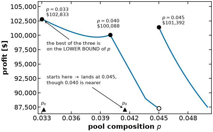
Only Options 1 and 2 are reproducible without further qualification. Option 3 is
nonconvex, and the profit reported for it is the profit at the initial point we
pinned. Changing bound_frac to 0.5 --- which changes nothing about the model ---
returns 101,392.16 instead. Whenever you tabulate the answer to a nonconvex problem,
the initialization belongs in the table with it.
Summary of the three options
One builder, three restrictions, three answers. The middle column is what was passed to
create_milk_model, so this is a table of restrictions --- not a table of unrelated
models.
summary = pd.DataFrame(
    [
        {
            "Option": "1. Local farms only",
            "L (blended)": ", ".join(local_farms),
            "R (pooled)": "(empty)",
            "Model class": "LP",
            "Profit": profit_1,
            "p": np.nan,
            "Catch": "leaves money on the table",
        },
        {
            "Option": "2. All farms, one truck each",
            "L (blended)": ", ".join(all_farms),
            "R (pooled)": "(empty)",
            "Model class": "LP",
            "Profit": profit_2,
            "p": np.nan,
            "Catch": "needs a second truck",
        },
        {
            "Option": "3. Remote farms pooled",
            "L (blended)": ", ".join(local_farms),
            "R (pooled)": ", ".join(remote_farms),
            "Model class": "bilinear NLP",
            "Profit": profit_3,
            "p": pyo.value(m3.p),
            "Catch": "nonconvex; bound_frac = 0.01",
        },
    ]
)
display(summary.round(4))# Regression guard. These three numbers are what this notebook is for; if a
# change to the builder moves one of them, that is the thing to notice first.
# Option 3's value is the one reached from bound_frac = 0.01 -- the other local
# solution, 101,392.16, is equally valid output from the same model.
for got, want, label in [
(profit_1, 81_000.00, "Option 1"),
(profit_2, 122_441.18, "Option 2"),
(profit_3, 102_833.33, "Option 3, bound_frac = 0.01"),
(profit_3_alt, 101_392.16, "Option 3, bound_frac = 0.50"),
]:
assert abs(got - want) < 0.01, f"{label}: {got:,.2f} != {want:,.2f}"
print(f"{label:<28} {got:>12,.2f}")Option 1 81,000.00
Option 2 122,441.18
Option 3, bound_frac = 0.01 102,833.33
Option 3, bound_frac = 0.50 101,392.16
Take away messages
Pooling recovers most of the value of the remote farms without a second truck. But the model that says so is nonconvex, and the number it reports depends on where the solver started.
A bilinear term --- a product of two decision variables --- is smooth but irreducibly nonconvex. Unlike , it cannot be reformulated away.
Report the initial point, or the option that determined it. A result you cannot reproduce is a result you cannot defend.
What can be done is to relax the bilinear term: replace it by a new variable bounded by linear functions of its factors. That gives a true upper bound on the profit, and tightening such bounds until they meet the optimum is what the global optimization lecture does.