Integer Programs - Optimization for Decision Science

# This code cell installs packages on Colab

import sys

if "google.colab" in sys.modules:
    !wget "https://raw.githubusercontent.com/ndcbe/optimization/main/notebooks/helper.py"
    import helper

    helper.easy_install()
else:
    sys.path.insert(0, "../")
    import helper
helper.set_plotting_style()

Optimizing Across Process Alternatives¶

Reference: Example 15.3 from Biegler, Grossmann, Westerberg (1997). See handout

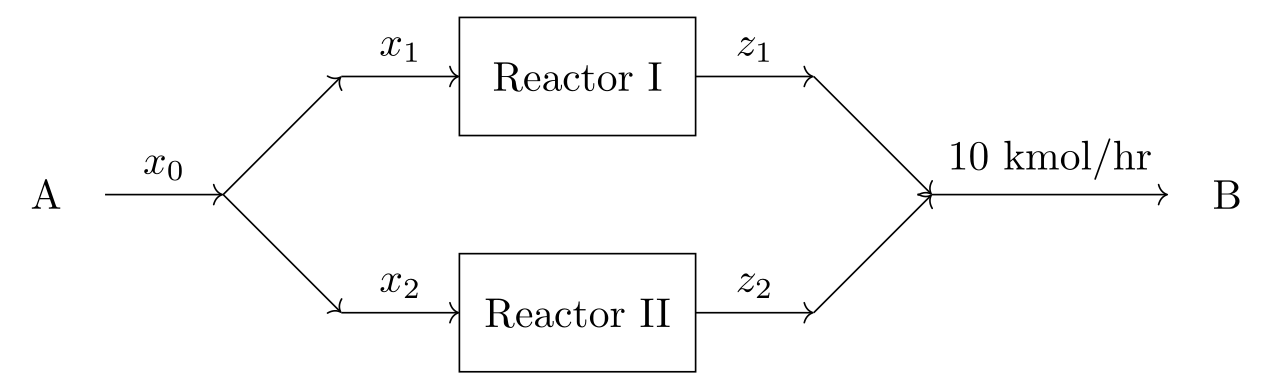
Assume that we have the choice of selecting two reactors (shown below) for the reaction $A \rightarrow B$ . Reactor I has a higher conversion (80%) but it is more expensive; reactor II has a lower conversion (66.7%) but is cheaper. The cost of feed $A$ is $5/kmol. Which process alternative (reactor I, reactor II, or both) has the minimum costs to make 10 kmol/hr of product B?

Let $x_r$ be the size (flowrate into) of reactor $r$ .

Continuous cost model: $C = \underbrace{a_r (x_r)^{0.6}}_{\text{reactor}} + \underbrace{5.0 x_r}_{\text{feed}}$

Develop the Optimization Model¶

Draw a Picture

Reactor selection superstructure: feed A splits between two reactors, products recombine to give B.

Sets

Parameters

Variables

Objective

Constraints

Degree of Freedom Analysis

Solve with Continuous Cost Model in Pyomo¶

We start by defining the model in Pyomo.

Units expose a problem in the cost model¶

Declaring units on this model does not just document it --- it fails. The reactor capital cost $a_r x_r^{0.6}$ has $a_r$ in $/hr and $x_r$ in kmol/hr, so the product comes out in $\mathrm{\$ \cdot kmol^{0.6} \, hr^{-1.6}}$ , not $/hr. Pyomo raises UnitsError and it is right to: a power law of a dimensioned quantity is not dimensionally homogeneous.

Economy-of-scale correlations always carry an implicit reference scale. Writing it down,

C_r = a_r \left( \frac{x_r}{x_{\mathrm{ref}}} \right)^{0.6}, \qquad x_{\mathrm{ref}} = 1~\mathrm{kmol/hr},

(1)

makes the base of the power dimensionless and the cost $/hr. The numbers do not change, because $x_{\mathrm{ref}} = 1$ --- but the units now check, and the reader can see which flowrate unit the fitted coefficients 5.5 and 4.0 belong to. That information was previously nowhere in the model.

import pyomo.environ as pyo
from pyomo.environ import units as u
from pyomo.util.check_units import assert_units_consistent

# Pyomo's unit library has kmol and hr but no money, so declare a currency.
u.load_definitions_from_strings(["USD = [currency]"])

nlp = pyo.ConcreteModel()

## Define sets
nlp.REACTORS = pyo.Set(initialize=range(1, 3))

## Define parameters (data)

# Cost coefficient of reactor r, a_r [USD/hr]
cost_coefficient = {1: 5.5, 2: 4.0}
nlp.reactor_cost = pyo.Param(
    nlp.REACTORS, initialize=cost_coefficient, units=u.USD / u.hr
)

# Required product rate, P [kmol B/hr]
nlp.product_flowrate = pyo.Param(initialize=10.0, units=u.kmol / u.hr)

# Conversion of reactor r, theta_r [kmol B/kmol A]
reactor_conversion = {1: 0.8, 2: 2 / 3}
nlp.conversion = pyo.Param(nlp.REACTORS, initialize=reactor_conversion)

# Price of feed A, c_f [USD/kmol]
nlp.feed_cost = pyo.Param(initialize=5.0, units=u.USD / u.kmol)

# Reference flowrate for the economy-of-scale term, x_ref [kmol/hr]
nlp.flowrate_ref = pyo.Param(initialize=1.0, units=u.kmol / u.hr)


## Define variables

# Total feed of A, x_0 in the notes [kmol/hr]
nlp.feed_flowrate = pyo.Var(domain=pyo.NonNegativeReals, units=u.kmol / u.hr)

# Feed into reactor r, x_r in the notes [kmol/hr]
nlp.reactor_feed = pyo.Var(
    nlp.REACTORS, domain=pyo.NonNegativeReals, units=u.kmol / u.hr
)

# Effluent leaving reactor r, z_r in the notes [kmol B/hr]
nlp.reactor_effluent = pyo.Var(
    nlp.REACTORS, domain=pyo.NonNegativeReals, units=u.kmol / u.hr
)

## Define constraints

# Add your solution here

## Define objective


# Total cost [USD/hr]. The exponent 0.6 is the economy-of-scale factor beta,
# applied to the flowrate scaled by x_ref so that the power is dimensionless.
@nlp.Objective()
def cost(b):
    return (
        sum(
            b.reactor_cost[r] * (b.reactor_feed[r] / b.flowrate_ref) ** (0.6)
            for r in b.REACTORS
        )
        + b.feed_cost * b.feed_flowrate
    )

# Inspect the model
nlp.pprint()

# Raises UnitsError if any constraint or the objective is dimensionally inconsistent
assert_units_consistent(nlp)

print("Units are consistent.")

1 Set Declarations
    REACTORS : Size=1, Index=None, Ordered=Insertion
        Key  : Dimen : Domain : Size : Members
        None :     1 :    Any :    2 : {1, 2}

5 Param Declarations
    conversion : Size=2, Index=REACTORS, Domain=Any, Default=None, Mutable=False
        Key : Value
          1 :                0.8
          2 : 0.6666666666666666
    feed_cost : Size=1, Index=None, Domain=Any, Default=None, Mutable=True, Units=USD/kmol
        Key  : Value
        None :   5.0
    flowrate_ref : Size=1, Index=None, Domain=Any, Default=None, Mutable=True, Units=kmol/h
        Key  : Value
        None :   1.0
    product_flowrate : Size=1, Index=None, Domain=Any, Default=None, Mutable=True, Units=kmol/h
        Key  : Value
        None :  10.0
    reactor_cost : Size=2, Index=REACTORS, Domain=Any, Default=None, Mutable=True, Units=USD/h
        Key : Value
          1 :   5.5
          2 :   4.0

3 Var Declarations
    feed_flowrate : Size=1, Index=None, Units=kmol/h
        Key  : Lower : Value : Upper : Fixed : Stale : Domain
        None :     0 :  None :  None : False :  True : NonNegativeReals
    reactor_effluent : Size=2, Index=REACTORS, Units=kmol/h
        Key : Lower : Value : Upper : Fixed : Stale : Domain
          1 :     0 :  None :  None : False :  True : NonNegativeReals
          2 :     0 :  None :  None : False :  True : NonNegativeReals
    reactor_feed : Size=2, Index=REACTORS, Units=kmol/h
        Key : Lower : Value : Upper : Fixed : Stale : Domain
          1 :     0 :  None :  None : False :  True : NonNegativeReals
          2 :     0 :  None :  None : False :  True : NonNegativeReals

1 Objective Declarations
    cost : Size=1, Index=None, Active=True
        Key  : Active : Sense    : Expression
        None :   True : minimize : reactor_cost[1]*(1/flowrate_ref*reactor_feed[1])**0.6 + reactor_cost[2]*(1/flowrate_ref*reactor_feed[2])**0.6 + feed_cost*feed_flowrate

3 Constraint Declarations
    inlet_split : Size=1, Index=None, Active=True
        Key  : Lower : Body                                                : Upper : Active
        None :   0.0 : feed_flowrate - (reactor_feed[1] + reactor_feed[2]) :   0.0 :   True
    mixer : Size=1, Index=None, Active=True
        Key  : Lower            : Body                                      : Upper            : Active
        None : product_flowrate : reactor_effluent[1] + reactor_effluent[2] : product_flowrate :   True
    reactor_performance : Size=2, Index=REACTORS, Active=True
        Key : Lower : Body                                                     : Upper : Active
          1 :   0.0 :                reactor_effluent[1] - 0.8*reactor_feed[1] :   0.0 :   True
          2 :   0.0 : reactor_effluent[2] - 0.6666666666666666*reactor_feed[2] :   0.0 :   True

13 Declarations: REACTORS reactor_cost product_flowrate conversion feed_cost flowrate_ref feed_flowrate reactor_feed reactor_effluent inlet_split reactor_performance mixer cost
Units are consistent.

# Mass balance over the splitter [kmol/hr]
@nlp.Constraint()
def inlet_split(b):
    return b.feed_flowrate == sum(b.reactor_feed[r] for r in b.REACTORS)


# Reactor conversion, z_r = theta_r * x_r [kmol B/hr]
@nlp.Constraint(nlp.REACTORS)
def reactor_performance(b, r):
    return b.reactor_effluent[r] == b.conversion[r] * b.reactor_feed[r]


# Mass balance over the mixer meets product requirements [kmol B/hr]
@nlp.Constraint()
def mixer(b):
    return b.product_flowrate == sum(b.reactor_effluent[r] for r in b.REACTORS)

Initialize to Favor Reaction 1 and Solve¶

def initialize(model, reactor_choice=1):
    """Initialize all of the variables in the model to demonstrate local solutions

    Arguments:
        model: Pyomo model
        reactor_choice: 1 or 2

    Returns:
        nothing

    Action:
        initializes model

    """

    # Guess 20 kmol/hr feed of A
    model.feed_flowrate = 20.0

    # Either assign all of the feed to reactor 1 or 2
    if reactor_choice == 1:
        model.reactor_feed[1] = 20.0
        model.reactor_feed[2] = 0
    elif reactor_choice == 2:
        model.reactor_feed[1] = 0
        model.reactor_feed[2] = 20.0
    else:
        raise ValueError("Argument reactor_choice needs value 1 or 2.")

    # Based on the feed assignments, calculate effluent flowrate
    for r in model.REACTORS:
        model.reactor_effluent[r] = model.reactor_feed[r]() * model.conversion[r]


initialize(nlp, reactor_choice=1)
nlp.pprint()

1 Set Declarations
    REACTORS : Size=1, Index=None, Ordered=Insertion
        Key  : Dimen : Domain : Size : Members
        None :     1 :    Any :    2 : {1, 2}

5 Param Declarations
    conversion : Size=2, Index=REACTORS, Domain=Any, Default=None, Mutable=False
        Key : Value
          1 :                0.8
          2 : 0.6666666666666666
    feed_cost : Size=1, Index=None, Domain=Any, Default=None, Mutable=True, Units=USD/kmol
        Key  : Value
        None :   5.0
    flowrate_ref : Size=1, Index=None, Domain=Any, Default=None, Mutable=True, Units=kmol/h
        Key  : Value
        None :   1.0
    product_flowrate : Size=1, Index=None, Domain=Any, Default=None, Mutable=True, Units=kmol/h
        Key  : Value
        None :  10.0
    reactor_cost : Size=2, Index=REACTORS, Domain=Any, Default=None, Mutable=True, Units=USD/h
        Key : Value
          1 :   5.5
          2 :   4.0

3 Var Declarations
    feed_flowrate : Size=1, Index=None, Units=kmol/h
        Key  : Lower : Value : Upper : Fixed : Stale : Domain
        None :     0 :  20.0 :  None : False : False : NonNegativeReals
    reactor_effluent : Size=2, Index=REACTORS, Units=kmol/h
        Key : Lower : Value : Upper : Fixed : Stale : Domain
          1 :     0 :  16.0 :  None : False : False : NonNegativeReals
          2 :     0 :   0.0 :  None : False : False : NonNegativeReals
    reactor_feed : Size=2, Index=REACTORS, Units=kmol/h
        Key : Lower : Value : Upper : Fixed : Stale : Domain
          1 :     0 :  20.0 :  None : False : False : NonNegativeReals
          2 :     0 :     0 :  None : False : False : NonNegativeReals

1 Objective Declarations
    cost : Size=1, Index=None, Active=True
        Key  : Active : Sense    : Expression
        None :   True : minimize : reactor_cost[1]*(1/flowrate_ref*reactor_feed[1])**0.6 + reactor_cost[2]*(1/flowrate_ref*reactor_feed[2])**0.6 + feed_cost*feed_flowrate

3 Constraint Declarations
    inlet_split : Size=1, Index=None, Active=True
        Key  : Lower : Body                                                : Upper : Active
        None :   0.0 : feed_flowrate - (reactor_feed[1] + reactor_feed[2]) :   0.0 :   True
    mixer : Size=1, Index=None, Active=True
        Key  : Lower            : Body                                      : Upper            : Active
        None : product_flowrate : reactor_effluent[1] + reactor_effluent[2] : product_flowrate :   True
    reactor_performance : Size=2, Index=REACTORS, Active=True
        Key : Lower : Body                                                     : Upper : Active
          1 :   0.0 :                reactor_effluent[1] - 0.8*reactor_feed[1] :   0.0 :   True
          2 :   0.0 : reactor_effluent[2] - 0.6666666666666666*reactor_feed[2] :   0.0 :   True

13 Declarations: REACTORS reactor_cost product_flowrate conversion feed_cost flowrate_ref feed_flowrate reactor_feed reactor_effluent inlet_split reactor_performance mixer cost

Now let’s solve the model.

solver = pyo.SolverFactory("ipopt")
results = solver.solve(nlp, tee=True)

Ipopt 3.13.2: 

******************************************************************************
This program contains Ipopt, a library for large-scale nonlinear optimization.
 Ipopt is released as open source code under the Eclipse Public License (EPL).
         For more information visit http://projects.coin-or.org/Ipopt

This version of Ipopt was compiled from source code available at
    https://github.com/IDAES/Ipopt as part of the Institute for the Design of
    Advanced Energy Systems Process Systems Engineering Framework (IDAES PSE
    Framework) Copyright (c) 2018-2019. See https://github.com/IDAES/idaes-pse.

This version of Ipopt was compiled using HSL, a collection of Fortran codes
    for large-scale scientific computation.  All technical papers, sales and
    publicity material resulting from use of the HSL codes within IPOPT must
    contain the following acknowledgement:
        HSL, a collection of Fortran codes for large-scale scientific
        computation. See http://www.hsl.rl.ac.uk.
******************************************************************************

This is Ipopt version 3.13.2, running with linear solver ma27.

Number of nonzeros in equality constraint Jacobian...:        9
Number of nonzeros in inequality constraint Jacobian.:        0
Number of nonzeros in Lagrangian Hessian.............:        2

Error evaluating "var =" definition -1: can't evaluate pow'(0,0.6).

ERROR: Solver (ipopt) returned non-zero return code (1)

ERROR: See the solver log above for diagnostic information.

---------------------------------------------------------------------------
ApplicationError                          Traceback (most recent call last)
Cell In[5], line 2
      1 solver = pyo.SolverFactory("ipopt")
----> 2 results = solver.solve(nlp, tee=True)

File ~/opt/anaconda3/envs/optimization_fall2026/lib/python3.13/site-packages/pyomo/opt/base/solvers.py:657, in OptSolver.solve(self, *args, **kwds)
    655     elif hasattr(_status, 'log') and _status.log:
    656         logger.error("Solver log:\n" + str(_status.log))
--> 657     raise ApplicationError("Solver (%s) did not exit normally" % self.name)
    658 solve_completion_time = time.time()
    659 if self._report_timing:

ApplicationError: Solver (ipopt) did not exit normally

What happened? 0^0.6 is fine --- it is 0. The derivative is not: $\frac{d}{dx}x^{0.6} = 0.6\,x^{-0.4} \to \infty$ as $x \to 0$ , and Ipopt needs it. Read the message again: can't evaluate pow'(0,0.6) --- note the prime. Work around? Let’s set the lower bound to something really small:

small_number = 1e-6
for r in nlp.REACTORS:

    # Set lower bound
    nlp.reactor_feed[r].setlb(small_number)

    # Adjust initial point if needed
    nlp.reactor_feed[r] = max(nlp.reactor_feed[r](), small_number)

nlp.pprint()

1 Set Declarations
    REACTORS : Size=1, Index=None, Ordered=Insertion
        Key  : Dimen : Domain : Size : Members
        None :     1 :    Any :    2 : {1, 2}

5 Param Declarations
    conversion : Size=2, Index=REACTORS, Domain=Any, Default=None, Mutable=False
        Key : Value
          1 :                0.8
          2 : 0.6666666666666666
    feed_cost : Size=1, Index=None, Domain=Any, Default=None, Mutable=True, Units=USD/kmol
        Key  : Value
        None :   5.0
    flowrate_ref : Size=1, Index=None, Domain=Any, Default=None, Mutable=True, Units=kmol/h
        Key  : Value
        None :   1.0
    product_flowrate : Size=1, Index=None, Domain=Any, Default=None, Mutable=True, Units=kmol/h
        Key  : Value
        None :  10.0
    reactor_cost : Size=2, Index=REACTORS, Domain=Any, Default=None, Mutable=True, Units=USD/h
        Key : Value
          1 :   5.5
          2 :   4.0

3 Var Declarations
    feed_flowrate : Size=1, Index=None, Units=kmol/h
        Key  : Lower : Value : Upper : Fixed : Stale : Domain
        None :     0 :  20.0 :  None : False : False : NonNegativeReals
    reactor_effluent : Size=2, Index=REACTORS, Units=kmol/h
        Key : Lower : Value : Upper : Fixed : Stale : Domain
          1 :     0 :  16.0 :  None : False : False : NonNegativeReals
          2 :     0 :   0.0 :  None : False : False : NonNegativeReals
    reactor_feed : Size=2, Index=REACTORS, Units=kmol/h
        Key : Lower : Value : Upper : Fixed : Stale : Domain
          1 : 1e-06 :  20.0 :  None : False : False : NonNegativeReals
          2 : 1e-06 : 1e-06 :  None : False : False : NonNegativeReals

1 Objective Declarations
    cost : Size=1, Index=None, Active=True
        Key  : Active : Sense    : Expression
        None :   True : minimize : reactor_cost[1]*(1/flowrate_ref*reactor_feed[1])**0.6 + reactor_cost[2]*(1/flowrate_ref*reactor_feed[2])**0.6 + feed_cost*feed_flowrate

3 Constraint Declarations
    inlet_split : Size=1, Index=None, Active=True
        Key  : Lower : Body                                                : Upper : Active
        None :   0.0 : feed_flowrate - (reactor_feed[1] + reactor_feed[2]) :   0.0 :   True
    mixer : Size=1, Index=None, Active=True
        Key  : Lower            : Body                                      : Upper            : Active
        None : product_flowrate : reactor_effluent[1] + reactor_effluent[2] : product_flowrate :   True
    reactor_performance : Size=2, Index=REACTORS, Active=True
        Key : Lower : Body                                                     : Upper : Active
          1 :   0.0 :                reactor_effluent[1] - 0.8*reactor_feed[1] :   0.0 :   True
          2 :   0.0 : reactor_effluent[2] - 0.6666666666666666*reactor_feed[2] :   0.0 :   True

13 Declarations: REACTORS reactor_cost product_flowrate conversion feed_cost flowrate_ref feed_flowrate reactor_feed reactor_effluent inlet_split reactor_performance mixer cost

Now let’s resolve:

solver = pyo.SolverFactory("ipopt")
results = solver.solve(nlp, tee=True)
assert pyo.check_optimal_termination(results), (
    f"Solve failed: status={results.solver.status}, "
    f"termination={results.solver.termination_condition}"
)

Ipopt 3.13.2: 

******************************************************************************
This program contains Ipopt, a library for large-scale nonlinear optimization.
 Ipopt is released as open source code under the Eclipse Public License (EPL).
         For more information visit http://projects.coin-or.org/Ipopt

This version of Ipopt was compiled from source code available at
    https://github.com/IDAES/Ipopt as part of the Institute for the Design of
    Advanced Energy Systems Process Systems Engineering Framework (IDAES PSE
    Framework) Copyright (c) 2018-2019. See https://github.com/IDAES/idaes-pse.

This version of Ipopt was compiled using HSL, a collection of Fortran codes
    for large-scale scientific computation.  All technical papers, sales and
    publicity material resulting from use of the HSL codes within IPOPT must
    contain the following acknowledgement:
        HSL, a collection of Fortran codes for large-scale scientific
        computation. See http://www.hsl.rl.ac.uk.
******************************************************************************

This is Ipopt version 3.13.2, running with linear solver ma27.

Number of nonzeros in equality constraint Jacobian...:        9
Number of nonzeros in inequality constraint Jacobian.:        0
Number of nonzeros in Lagrangian Hessian.............:        2

Total number of variables............................:        5
                     variables with only lower bounds:        5
                variables with lower and upper bounds:        0
                     variables with only upper bounds:        0
Total number of equality constraints.................:        4
Total number of inequality constraints...............:        0
        inequality constraints with only lower bounds:        0
   inequality constraints with lower and upper bounds:        0
        inequality constraints with only upper bounds:        0

iter    objective    inf_pr   inf_du lg(mu)  ||d||  lg(rg) alpha_du alpha_pr  ls
   0  1.3344037e+02 6.01e+00 8.35e-01  -1.0 0.00e+00    -  0.00e+00 0.00e+00   0
   1  8.9515896e+01 1.78e-15 1.12e+01  -1.0 7.77e+00    -  4.39e-02 1.00e+00f  1
   2  8.9555393e+01 0.00e+00 5.56e+00  -1.0 2.22e-02    -  9.98e-01 5.00e-01f  2
   3  8.9541585e+01 2.78e-17 2.24e-05  -1.0 3.90e-03    -  1.00e+00 1.00e+00f  1
   4  8.7593746e+01 1.78e-17 5.53e+00  -2.5 5.40e-01    -  9.89e-01 6.15e-01f  1
   5  8.7593068e+01 0.00e+00 1.75e-01  -2.5 1.74e-05   4.0 1.00e+00 1.00e+00f  1
   6  8.7589190e+01 1.78e-15 2.20e-02  -2.5 9.70e-05    -  1.00e+00 1.00e+00f  1
   7  8.7533830e+01 8.16e-20 8.54e+01  -3.8 1.31e-03    -  1.00e+00 6.29e-01f  1
   8  8.7542212e+01 1.78e-15 2.05e+02  -3.8 8.17e-05    -  2.27e-03 5.00e-01f  2
   9  8.7536537e+01 3.39e-21 1.89e+01  -3.8 3.29e-05   5.3 1.00e+00 1.00e+00f  1
iter    objective    inf_pr   inf_du lg(mu)  ||d||  lg(rg) alpha_du alpha_pr  ls
  10  8.7535629e+01 1.78e-15 7.28e+00  -3.8 6.69e-06   5.8 1.00e+00 5.00e-01f  2
  11  8.7536094e+01 1.78e-15 9.18e-01  -3.8 1.64e-06    -  1.00e+00 1.00e+00f  1
  12  8.7536019e+01 0.00e+00 1.80e-02  -3.8 2.76e-07    -  1.00e+00 1.00e+00f  1
  13  8.7536022e+01 1.78e-15 2.74e-05  -3.8 1.04e-08    -  1.00e+00 1.00e+00f  1
  14  8.7533756e+01 1.78e-15 3.24e+01  -5.7 1.03e-05    -  1.00e+00 5.98e-01f  1
  15  8.7533783e+01 1.78e-15 5.52e-02  -5.7 4.47e-08    -  1.00e+00 1.00e+00f  1
  16  8.7533768e+01 1.78e-15 1.74e-02  -5.7 2.57e-08    -  1.00e+00 1.00e+00f  1
  17  8.7533768e+01 1.78e-15 1.13e-07  -5.7 6.42e-11    -  1.00e+00 1.00e+00h  1
  18  8.7533756e+01 1.78e-15 6.33e-02  -8.6 1.93e-08    -  1.00e+00 9.76e-01f  1
  19  8.7533756e+01 1.06e-22 1.79e-08  -8.6 2.50e-11    -  1.00e+00 1.00e+00f  1
iter    objective    inf_pr   inf_du lg(mu)  ||d||  lg(rg) alpha_du alpha_pr  ls
  20  8.7533756e+01 1.78e-15 7.27e-09  -9.0 1.59e-11    -  1.00e+00 1.00e+00f  1

Number of Iterations....: 20

                                   (scaled)                 (unscaled)
Objective...............:   1.4519923360965409e+01    8.7533756344723201e+01
Dual infeasibility......:   7.2654700034036068e-09    4.3800085248214534e-08
Constraint violation....:   1.7763568394002505e-15    1.7763568394002505e-15
Complementarity.........:   9.0911618236617630e-10    5.4806318475633307e-09
Overall NLP error.......:   7.2654700034036068e-09    4.3800085248214534e-08


Number of objective function evaluations             = 30
Number of objective gradient evaluations             = 21
Number of equality constraint evaluations            = 30
Number of inequality constraint evaluations          = 0
Number of equality constraint Jacobian evaluations   = 21
Number of inequality constraint Jacobian evaluations = 0
Number of Lagrangian Hessian evaluations             = 20
Total CPU secs in IPOPT (w/o function evaluations)   =      0.002
Total CPU secs in NLP function evaluations           =      0.000

EXIT: Optimal Solution Found.

Now we can print the variable names and values:

def print_solution(model):
    """Print variable names and values

    Arguments:
        model: Pyomo model

    """

    print("Variable Names\t\tValue")
    for c in model.component_data_objects(pyo.Var):
        print(c.name, "\t\t", pyo.value(c))

    print("\nObjective Name\t\tValue")
    for c in model.component_data_objects(pyo.Objective):
        print(c.name, "\t\t", pyo.value(c))


print_solution(nlp)

Variable Names		Value
feed_flowrate 		 12.50000016500151
reactor_feed[1] 		 12.499999174992452
reactor_feed[2] 		 1e-06
reactor_effluent[1] 		 9.999999339993963
reactor_effluent[2] 		 6.600060378065732e-07

Objective Name		Value
cost 		 87.53376237988246

Initialize to Favor Reaction 2 and Solve¶

# Initialize
initialize(nlp, reactor_choice=2)

# Correct for bound
# Note: I would have put this in the initialize function but I wanted to show
# the error in class
for r in nlp.REACTORS:
    # Adjust initial point if needed
    nlp.reactor_feed[r] = max(nlp.reactor_feed[r](), small_number)

results = solver.solve(nlp, tee=True)
assert pyo.check_optimal_termination(results), (
    f"Solve failed: status={results.solver.status}, "
    f"termination={results.solver.termination_condition}"
)
print_solution(nlp)

WARNING (W1002): Setting Var 'reactor_feed[1]' to a numeric value `0` outside
the bounds (1e-06, None).
    See also https://pyomo.readthedocs.io/en/stable/errors.html#w1002

Ipopt 3.13.2: 

******************************************************************************
This program contains Ipopt, a library for large-scale nonlinear optimization.
 Ipopt is released as open source code under the Eclipse Public License (EPL).
         For more information visit http://projects.coin-or.org/Ipopt

This version of Ipopt was compiled from source code available at
    https://github.com/IDAES/Ipopt as part of the Institute for the Design of
    Advanced Energy Systems Process Systems Engineering Framework (IDAES PSE
    Framework) Copyright (c) 2018-2019. See https://github.com/IDAES/idaes-pse.

This version of Ipopt was compiled using HSL, a collection of Fortran codes
    for large-scale scientific computation.  All technical papers, sales and
    publicity material resulting from use of the HSL codes within IPOPT must
    contain the following acknowledgement:
        HSL, a collection of Fortran codes for large-scale scientific
        computation. See http://www.hsl.rl.ac.uk.
******************************************************************************

This is Ipopt version 3.13.2, running with linear solver ma27.

Number of nonzeros in equality constraint Jacobian...:        9
Number of nonzeros in inequality constraint Jacobian.:        0
Number of nonzeros in Lagrangian Hessian.............:        2

Total number of variables............................:        5
                     variables with only lower bounds:        5
                variables with lower and upper bounds:        0
                     variables with only upper bounds:        0
Total number of equality constraints.................:        4
Total number of inequality constraints...............:        0
        inequality constraints with only lower bounds:        0
   inequality constraints with lower and upper bounds:        0
        inequality constraints with only upper bounds:        0

iter    objective    inf_pr   inf_du lg(mu)  ||d||  lg(rg) alpha_du alpha_pr  ls
   0  1.2448375e+02 3.34e+00 8.57e-01  -1.0 0.00e+00    -  0.00e+00 0.00e+00   0
   1  9.7212017e+01 1.78e-15 9.39e+00  -1.0 5.30e+00    -  6.57e-02 1.00e+00f  1
   2  9.9691054e+01 2.22e-16 2.07e+00  -1.0 2.28e+00    -  1.39e-01 1.00e+00f  1
   3  9.9758192e+01 1.78e-15 6.79e-04  -1.0 2.43e-01    -  1.00e+00 1.00e+00f  1
   4  9.9364492e+01 1.78e-15 2.03e-02  -1.7 9.59e-01  -2.0 9.78e-01 1.00e+00f  1
   5  9.5513279e+01 2.39e-17 3.07e+00  -2.5 2.56e+00  -1.6 1.00e+00 7.26e-01f  1
   6  9.5434966e+01 1.78e-15 1.31e+00  -2.5 2.97e-03   2.5 1.00e+00 1.00e+00f  1
   7  9.5393290e+01 2.17e-19 1.79e+01  -2.5 4.95e-02   2.0 1.00e+00 2.31e-02f  2
   8  9.5392828e+01 0.00e+00 1.60e-04  -2.5 1.08e-05    -  1.00e+00 1.00e+00f  1
   9  9.5311712e+01 3.70e-20 8.53e+01  -3.8 1.85e-03    -  1.00e+00 6.16e-01f  1
iter    objective    inf_pr   inf_du lg(mu)  ||d||  lg(rg) alpha_du alpha_pr  ls
  10  9.5322431e+01 1.78e-15 1.70e+02  -3.8 1.78e-04    -  1.20e-03 2.50e-01f  3
  11  9.5318416e+01 1.69e-20 9.28e+01  -3.8 4.85e-05   5.1 1.00e+00 4.60e-01f  2
  12  9.5315798e+01 1.86e-20 2.73e+02  -3.8 4.07e-04    -  1.00e+00 2.74e-02f  2
  13  9.5315678e+01 0.00e+00 1.44e-02  -3.8 4.39e-07    -  1.00e+00 1.00e+00f  1
  14  9.5314637e+01 0.00e+00 1.31e+00  -3.8 3.55e-06    -  1.00e+00 1.00e+00f  1
  15  9.5314724e+01 1.78e-15 1.37e-02  -3.8 2.76e-07    -  1.00e+00 1.00e+00f  1
  16  9.5314720e+01 1.78e-15 2.30e-05  -3.8 1.16e-08    -  1.00e+00 1.00e+00h  1
  17  9.5311597e+01 1.78e-15 3.25e+01  -5.7 1.25e-05    -  1.00e+00 5.96e-01f  1
  18  9.5311634e+01 1.78e-15 5.58e-02  -5.7 5.39e-08    -  1.00e+00 1.00e+00f  1
  19  9.5311613e+01 1.06e-22 1.77e-02  -5.7 3.11e-08    -  1.00e+00 1.00e+00f  1
iter    objective    inf_pr   inf_du lg(mu)  ||d||  lg(rg) alpha_du alpha_pr  ls
  20  9.5311612e+01 1.06e-22 1.14e-07  -5.7 7.73e-11    -  1.00e+00 1.00e+00h  1
  21  9.5311597e+01 1.78e-15 5.31e-02  -8.6 2.32e-08    -  1.00e+00 9.76e-01f  1
  22  9.5311597e+01 1.78e-15 1.80e-08  -8.6 3.00e-11    -  1.00e+00 1.00e+00f  1
  23  9.5311597e+01 1.78e-15 7.30e-09  -9.0 1.91e-11    -  1.00e+00 1.00e+00h  1

Number of Iterations....: 23

                                   (scaled)                 (unscaled)
Objective...............:   1.1498251558692399e+01    9.5311596851998971e+01
Dual infeasibility......:   7.2961370278790127e-09    6.0479323089120971e-08
Constraint violation....:   1.7763568394002505e-15    1.7763568394002505e-15
Complementarity.........:   9.0911629856797057e-10    7.5358697536224235e-09
Overall NLP error.......:   7.2961370278790127e-09    6.0479323089120971e-08


Number of objective function evaluations             = 32
Number of objective gradient evaluations             = 24
Number of equality constraint evaluations            = 32
Number of inequality constraint evaluations          = 0
Number of equality constraint Jacobian evaluations   = 24
Number of inequality constraint Jacobian evaluations = 0
Number of Lagrangian Hessian evaluations             = 23
Total CPU secs in IPOPT (w/o function evaluations)   =      0.002
Total CPU secs in NLP function evaluations           =      0.000

EXIT: Optimal Solution Found.

Variable Names		Value
feed_flowrate 		 14.999999801998188
reactor_feed[1] 		 1e-06
reactor_feed[2] 		 14.99999881198911
reactor_effluent[1] 		 7.92007260585095e-07
reactor_effluent[2] 		 9.99999920799274

Objective Name		Value
cost 		 95.31160515032713

Compare Solutions¶

	Solution 1	Solution 2
Feed Flowrate (kmol/hr)	12.50	15.00
Reactor 1 Feed (kmol/hr)	12.50	0
Reactor 2 Feed (kmol/hr)	0	15.00
Reactor 1 Effluent (kmol/hr)	10.00	0
Reactor 2 Effluent (kmol/hr)	0	10.00
Cost ($/hr)	87.53	95.31

Which solution is better? Why are there multiple solutions?

Why there are two solutions, as one picture¶

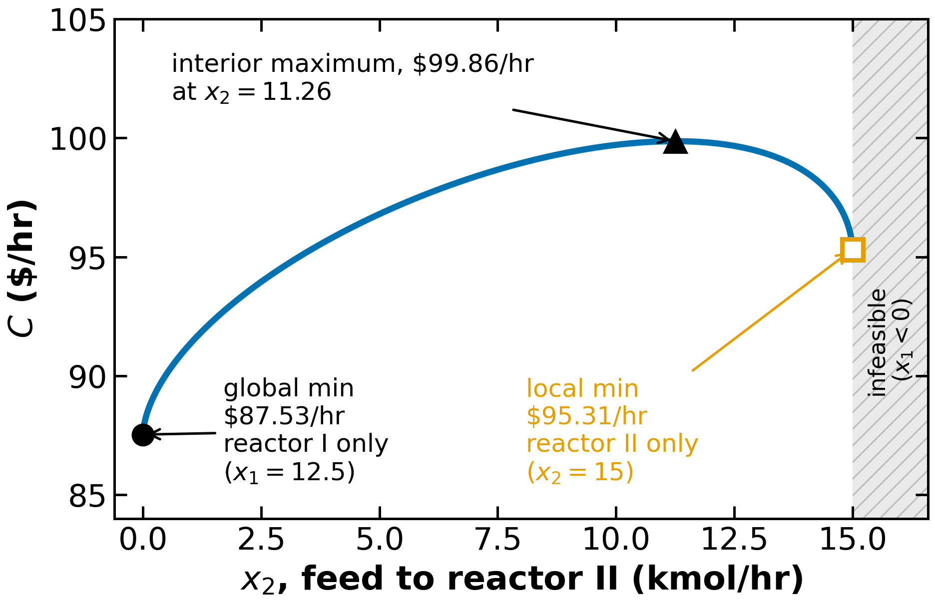
Cost along the mass balance as a function of the feed to reactor II: a concave curve on a segment, with local minima at both endpoints and a maximum in the interior.

Eliminating $x_1$ through $0.8 x_1 + (2/3) x_2 = 10$ leaves the cost a function of $x_2$ alone on the segment $0 \le x_2 \le 15$ . Because each $x^{0.6}$ term is concave, the cost is concave, so its minima sit at the two endpoints — use reactor I only, or use reactor II only — and its maximum is in the interior. Both endpoints satisfy the KKT conditions, so a local solver returns whichever one the initial guess was nearer. That is precisely what the two runs above did.

Rendered from figures/plots/reactor-concave-local-minima.py, and the same image printed in the course pack. It re-derives the curve with numpy rather than Pyomo, so regenerating it needs no solver binary. It recomputes Biegler, Grossmann & Westerberg (1997) Figure 15.12, p. 510. With $\theta_2 = 2/3$ the right-hand endpoint is $x_2 = 15$ exactly and $C = \$95.31$ /hr, matching their printed 95.3; the interior maximum recomputes to $x_2 = 11.26$ against their hand-drawn 11.4.

Linearized Discrete Cost Model¶

We want to modify the model to:

Easily find the best global solution (reduce impacts of initialization)
Account for the fact there is a minimum reactor size we can purchase

The linearized cost model, as one picture¶

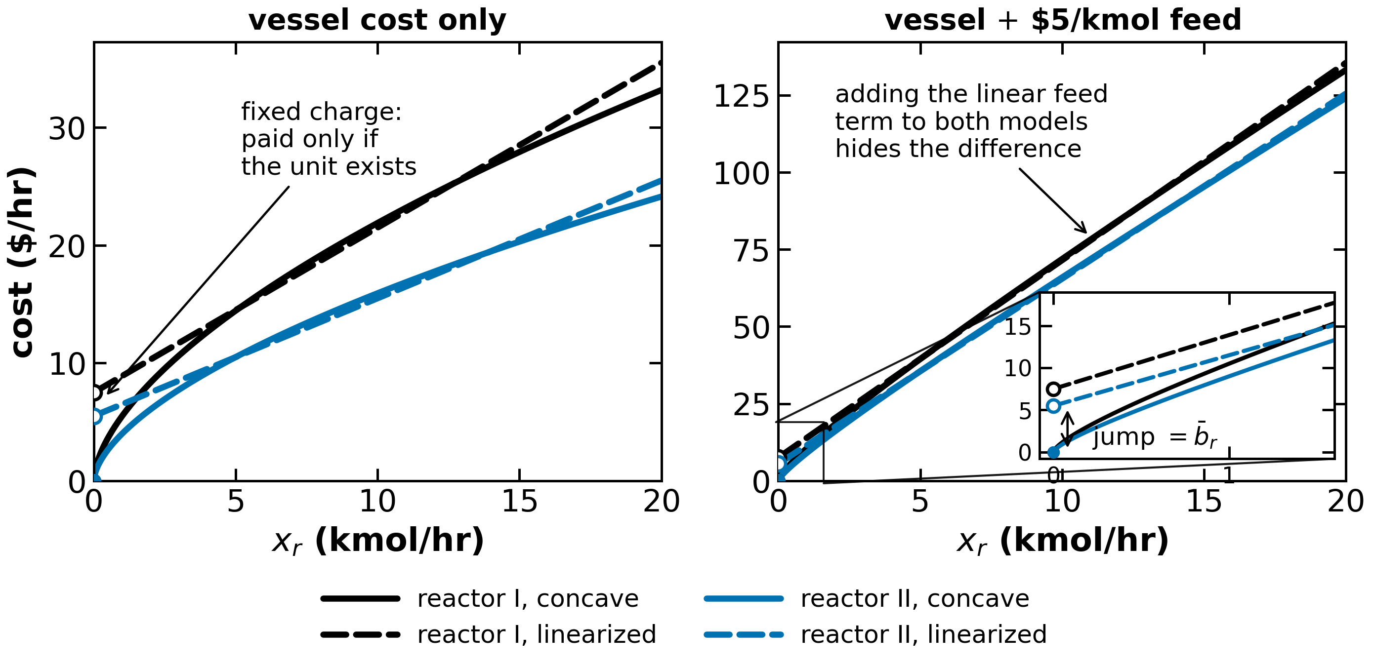
Fixed-charge linearization against the concave power law, both reactors: left, vessel cost only; right, with the $5/kmol feed added. The linearized model is discontinuous at zero feed.

Rendered from figures/plots/reactor-cost-linearization.py, and the same image printed in the course pack, so the handout and the website cannot drift apart. The left panel is Biegler, Grossmann & Westerberg, Systematic Methods of Chemical Process Design (1997), Figure 15.13, p. 511; the right panel is the cell below.

Note the jump at $x_r = 0$ : the fixed charge is paid only if the unit is built. That discontinuity is exactly what a binary variable is for.

Run the cell below to reproduce the right panel and change the constants yourself. (It plots only the total cost, so the two models nearly coincide — the feed term is linear in both.)

import matplotlib.pyplot as plt
import numpy as np

feed = np.linspace(0, 20, 101)

# Price of feed A, c_f [USD/kmol] -- the same for both reactors
c_feed = 5

for reactor in [1, 2]:

    if reactor == 1:
        c = 5.5
        c_linear = 6.4
        c_fixed = 7.5
        color = "r"
    elif reactor == 2:
        c = 4.0
        c_linear = 6.0
        c_fixed = 5.5
        color = "b"
    else:
        break

    cost_continuous = c * (feed) ** (0.6) + c_feed * feed
    cost_linearized = c_linear * feed + c_fixed

    plt.plot(
        feed,
        cost_continuous,
        label="Reactor " + str(reactor) + " (continuous)",
        color=color,
        linestyle="-",
    )
    plt.plot(
        feed,
        cost_linearized,
        label="Reactor " + str(reactor) + " (linearized)",
        color=color,
        linestyle="--",
    )

plt.legend()
plt.xlabel("Feed Flowrate (kmol/hr)")
plt.ylabel(r"Cost (\$/hr)")
plt.show()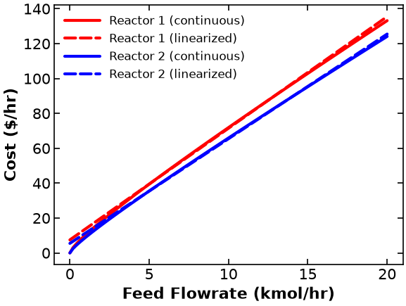

Define binary variable:

$y_r = \begin{cases} 1 & \text{if reactor } r \text{ is selected} \\ 0 & \text{otherwise} \end{cases}$

Add logical constraints to include the maximum flowrate (20 kmol/hr):

$x_r \leq 20 y_r, \quad \forall r \in \mathcal{R}$

Thus if $y_r = 0$ , then $x_r = 0$

Finally, we can define the new linearized reactor cost model:

\begin{align*} \text{Reactor I:} \quad & 7.5 y_1 + 1.4 x_1 \\ \text{Reactor II:} \quad & 5.5 y_2 + 1.0 x_2 \end{align*}

(2)

Recall that $x_0 = x_1 + x_2$ . Thus, the feed cost is $5x_0 = 5 x_1 + 5 x_2$ .

Putting this all together gives the following MILP optimization problem:

\begin{align*} \min_{x,y} \quad & C = 7.5 y_1 + 6.4 x_1 + 5.5 y_2 + 6.0 x_2 \\ \text{s.t.} \quad & 0.8 x_1 + (2/3) x_2 = 10 \\ & x_1 - 20 y_1 \leq 0 \\ & x_2 - 20 y_2 \leq 0 \\ & x_1, x_2 \geq 0, \quad y_1, y_2 \in \{0, 1\} \end{align*}

(3)

Enumerate the solutions¶

As an illustration, enumerate through the following four options:

No reactor
Reactor I only
Reactor II only
Reactor I and II only

For each option, ask:

Are the constraints feasible?
What is the objective?

Reactor 1	Reactor 2	Cost
0	0	infeasible
1	0	87.5
0	1	95.5
1	1	93.0

Solve with Pyomo¶

Create and inspect the model.

milp = pyo.ConcreteModel()

## Define sets
milp.REACTORS = pyo.Set(initialize=range(1, 3))

## Define parameters (data)

# Big-M throughput limit, M [kmol/hr]
milp.max_flowrate = pyo.Param(initialize=20.0, units=u.kmol / u.hr)

# Marginal (linear) cost of reactor r, abar_r [USD/kmol]
cost_coefficient1 = {1: 1.4, 2: 1.0}
milp.reactor_cost_linear = pyo.Param(
    milp.REACTORS, initialize=cost_coefficient1, units=u.USD / u.kmol
)

# Fixed charge for selecting reactor r, bbar_r [USD/hr]
cost_coefficient2 = {1: 7.5, 2: 5.5}
milp.reactor_cost_fixed = pyo.Param(
    milp.REACTORS, initialize=cost_coefficient2, units=u.USD / u.hr
)

# Required product rate, P [kmol B/hr]
milp.product_flowrate = pyo.Param(initialize=10.0, units=u.kmol / u.hr)

# Conversion of reactor r, theta_r [kmol B/kmol A]
reactor_conversion = {1: 0.8, 2: 2 / 3}
milp.conversion = pyo.Param(milp.REACTORS, initialize=reactor_conversion)

# Price of feed A, c_f [USD/kmol]
milp.feed_cost = pyo.Param(initialize=5.0, units=u.USD / u.kmol)


## Define variables

# Total feed of A, x_0 in the notes [kmol/hr]
milp.feed_flowrate = pyo.Var(
    domain=pyo.NonNegativeReals, bounds=(0, milp.max_flowrate), units=u.kmol / u.hr
)

# Feed into reactor r, x_r in the notes [kmol/hr]
milp.reactor_feed = pyo.Var(
    milp.REACTORS,
    domain=pyo.NonNegativeReals,
    bounds=(0, milp.max_flowrate),
    units=u.kmol / u.hr,
)

# Effluent leaving reactor r, z_r in the notes [kmol B/hr]
milp.reactor_effluent = pyo.Var(
    milp.REACTORS, domain=pyo.NonNegativeReals, units=u.kmol / u.hr
)

# Binary variables: y_r = 1 if reactor r is selected
# Add your solution here

## Define constraints


# Mass balance over the splitter [kmol/hr]
@milp.Constraint()
def inlet_split(b):
    return b.feed_flowrate == sum(b.reactor_feed[r] for r in b.REACTORS)


# Reactor conversion, z_r = theta_r * x_r [kmol B/hr]
@milp.Constraint(milp.REACTORS)
def reactor_performance(b, r):
    return b.reactor_effluent[r] == b.conversion[r] * b.reactor_feed[r]


# Mass balance over the mixer meets product requirements [kmol B/hr]
@milp.Constraint()
def mixer(b):
    return b.product_flowrate == sum(b.reactor_effluent[r] for r in b.REACTORS)


# Big-M logical constraint, x_r <= M * y_r [kmol/hr]
# Add your solution here

## Define objective


# BGW fold the feed price into each flow coefficient, abar_r + c_f = 6.4
# and 6.0; here the two terms are kept separate.
# Total cost [USD/hr]
# Add your solution here

# Inspect the model
milp.pprint()

# Raises UnitsError if any constraint or the objective is dimensionally inconsistent
assert_units_consistent(milp)

print("Units are consistent.")

1 Set Declarations
    REACTORS : Size=1, Index=None, Ordered=Insertion
        Key  : Dimen : Domain : Size : Members
        None :     1 :    Any :    2 : {1, 2}

6 Param Declarations
    conversion : Size=2, Index=REACTORS, Domain=Any, Default=None, Mutable=False
        Key : Value
          1 :                0.8
          2 : 0.6666666666666666
    feed_cost : Size=1, Index=None, Domain=Any, Default=None, Mutable=True, Units=USD/kmol
        Key  : Value
        None :   5.0
    max_flowrate : Size=1, Index=None, Domain=Any, Default=None, Mutable=True, Units=kmol/h
        Key  : Value
        None :  20.0
    product_flowrate : Size=1, Index=None, Domain=Any, Default=None, Mutable=True, Units=kmol/h
        Key  : Value
        None :  10.0
    reactor_cost_fixed : Size=2, Index=REACTORS, Domain=Any, Default=None, Mutable=True, Units=USD/h
        Key : Value
          1 :   7.5
          2 :   5.5
    reactor_cost_linear : Size=2, Index=REACTORS, Domain=Any, Default=None, Mutable=True, Units=USD/kmol
        Key : Value
          1 :   1.4
          2 :   1.0

4 Var Declarations
    feed_flowrate : Size=1, Index=None, Units=kmol/h
        Key  : Lower : Value : Upper : Fixed : Stale : Domain
        None :     0 :  None :  20.0 : False :  True : NonNegativeReals
    reactor_boolean : Size=2, Index=REACTORS
        Key : Lower : Value : Upper : Fixed : Stale : Domain
          1 :     0 :  None :     1 : False :  True : Binary
          2 :     0 :  None :     1 : False :  True : Binary
    reactor_effluent : Size=2, Index=REACTORS, Units=kmol/h
        Key : Lower : Value : Upper : Fixed : Stale : Domain
          1 :     0 :  None :  None : False :  True : NonNegativeReals
          2 :     0 :  None :  None : False :  True : NonNegativeReals
    reactor_feed : Size=2, Index=REACTORS, Units=kmol/h
        Key : Lower : Value : Upper : Fixed : Stale : Domain
          1 :     0 :  None :  20.0 : False :  True : NonNegativeReals
          2 :     0 :  None :  20.0 : False :  True : NonNegativeReals

1 Objective Declarations
    cost : Size=1, Index=None, Active=True
        Key  : Active : Sense    : Expression
        None :   True : minimize : reactor_cost_linear[1]*reactor_feed[1] + reactor_cost_fixed[1]*reactor_boolean[1] + reactor_cost_linear[2]*reactor_feed[2] + reactor_cost_fixed[2]*reactor_boolean[2] + feed_cost*feed_flowrate

4 Constraint Declarations
    inlet_split : Size=1, Index=None, Active=True
        Key  : Lower : Body                                                : Upper : Active
        None :   0.0 : feed_flowrate - (reactor_feed[1] + reactor_feed[2]) :   0.0 :   True
    mixer : Size=1, Index=None, Active=True
        Key  : Lower            : Body                                      : Upper            : Active
        None : product_flowrate : reactor_effluent[1] + reactor_effluent[2] : product_flowrate :   True
    reactor_performance : Size=2, Index=REACTORS, Active=True
        Key : Lower : Body                                                     : Upper : Active
          1 :   0.0 :                reactor_effluent[1] - 0.8*reactor_feed[1] :   0.0 :   True
          2 :   0.0 : reactor_effluent[2] - 0.6666666666666666*reactor_feed[2] :   0.0 :   True
    toggle_reactor : Size=2, Index=REACTORS, Active=True
        Key : Lower : Body                                              : Upper : Active
          1 :  -Inf : reactor_feed[1] - max_flowrate*reactor_boolean[1] :   0.0 :   True
          2 :  -Inf : reactor_feed[2] - max_flowrate*reactor_boolean[2] :   0.0 :   True

16 Declarations: REACTORS max_flowrate reactor_cost_linear reactor_cost_fixed product_flowrate conversion feed_cost feed_flowrate reactor_feed reactor_effluent reactor_boolean inlet_split reactor_performance mixer toggle_reactor cost
Units are consistent.

# Binary variables: y_r = 1 if reactor r is selected
milp.reactor_boolean = pyo.Var(milp.REACTORS, domain=pyo.Binary)


# Big-M logical constraint, x_r <= M * y_r [kmol/hr]
@milp.Constraint(milp.REACTORS)
def toggle_reactor(b, r):
    return b.reactor_feed[r] <= b.reactor_boolean[r] * b.max_flowrate


# Total cost [USD/hr]
@milp.Objective()
def cost(b):
    return (
        sum(
            b.reactor_cost_linear[r] * b.reactor_feed[r]
            + b.reactor_cost_fixed[r] * b.reactor_boolean[r]
            for r in b.REACTORS
        )
        + b.feed_cost * b.feed_flowrate
    )

Solve the model using cbc, bonmin, gurobi (need license), or cplex (need license).

# Set solver
# solver = pyo.SolverFactory('gurobi')
# solver = pyo.SolverFactory('glpk')
solver = pyo.SolverFactory("cbc")
# solver = pyo.SolverFactory('bonmin')

# Add your solution here

print_solution(milp)

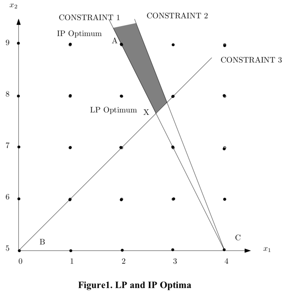
Is rounding good enough?¶

Linear Program (Relaxation)¶

\begin{align}\min_{x_1,x_2} \quad & x_2 \\ \mathrm{s.t.} \quad & 2 x_1 + x_2 \geq 13 \\ & 5 x_1 + 2 x_2 \leq 30 \\ & -x_1 + x_2 \geq 5 \\ & x_1, x_2 \geq 0 \end{align}

(4)

import pyomo.environ as pyo

m = pyo.ConcreteModel()

# Declare variables with bounds
m.x1 = pyo.Var(domain=pyo.NonNegativeReals)
m.x2 = pyo.Var(domain=pyo.NonNegativeReals)

# Constraint 1
m.con1 = pyo.Constraint(expr=2 * m.x1 + m.x2 >= 13)

# Constraint 2
m.con2 = pyo.Constraint(expr=5 * m.x1 + 2 * m.x2 <= 30)

# Constraint 3
m.con3 = pyo.Constraint(expr=-m.x1 + m.x2 >= 5)

# Objective
m.obj = pyo.Objective(expr=m.x2)

# Print model
m.pprint()

2 Var Declarations
    x1 : Size=1, Index=None
        Key  : Lower : Value : Upper : Fixed : Stale : Domain
        None :     0 :  None :  None : False :  True : NonNegativeReals
    x2 : Size=1, Index=None
        Key  : Lower : Value : Upper : Fixed : Stale : Domain
        None :     0 :  None :  None : False :  True : NonNegativeReals

1 Objective Declarations
    obj : Size=1, Index=None, Active=True
        Key  : Active : Sense    : Expression
        None :   True : minimize :         x2

3 Constraint Declarations
    con1 : Size=1, Index=None, Active=True
        Key  : Lower : Body      : Upper : Active
        None :  13.0 : 2*x1 + x2 :  +Inf :   True
    con2 : Size=1, Index=None, Active=True
        Key  : Lower : Body        : Upper : Active
        None :  -Inf : 5*x1 + 2*x2 :  30.0 :   True
    con3 : Size=1, Index=None, Active=True
        Key  : Lower : Body      : Upper : Active
        None :   5.0 : - x1 + x2 :  +Inf :   True

6 Declarations: x1 x2 con1 con2 con3 obj

# Set solver
# solver = pyo.SolverFactory('gurobi')
# solver = pyo.SolverFactory('glpk')
# solver = pyo.SolverFactory('ipopt')
solver = pyo.SolverFactory("cbc")


# Solve
results = solver.solve(m, tee=True)
assert pyo.check_optimal_termination(results), (
    f"Solve failed: status={results.solver.status}, "
    f"termination={results.solver.termination_condition}"
)

# Print solution
print(" ")
print("x1 = ", pyo.value(m.x1))
print("x2 = ", pyo.value(m.x2))

Welcome to the CBC MILP Solver 
Version: 2.10.10 
Build Date: Jun  7 2023 

command line - /Users/adowling/.idaes/bin/cbc -printingOptions all -import /var/folders/3w/vr4xmyqs451dg23xk88pqcg00000gq/T/tmp92qpkxje.pyomo.lp -stat=1 -solve -solu /var/folders/3w/vr4xmyqs451dg23xk88pqcg00000gq/T/tmp92qpkxje.pyomo.soln (default strategy 1)
Option for printingOptions changed from normal to all
Presolve 3 (0) rows, 2 (0) columns and 6 (0) elements
Statistics for presolved model


Problem has 3 rows, 2 columns (1 with objective) and 6 elements
Column breakdown:
2 of type 0.0->inf, 0 of type 0.0->up, 0 of type lo->inf, 
0 of type lo->up, 0 of type free, 0 of type fixed, 
0 of type -inf->0.0, 0 of type -inf->up, 0 of type 0.0->1.0 
Row breakdown:
0 of type E 0.0, 0 of type E 1.0, 0 of type E -1.0, 
0 of type E other, 0 of type G 0.0, 0 of type G 1.0, 
2 of type G other, 0 of type L 0.0, 0 of type L 1.0, 
1 of type L other, 0 of type Range 0.0->1.0, 0 of type Range other, 
0 of type Free 
Presolve 3 (0) rows, 2 (0) columns and 6 (0) elements
0  Obj 0 Primal inf 11.5 (2)
2  Obj 7.6666667
Optimal - objective value 7.6666667
Optimal objective 7.666666667 - 2 iterations time 0.002
Total time (CPU seconds):       0.00   (Wallclock seconds):       0.00

 
x1 =  2.6666667
x2 =  7.6666667

Rounding¶

With your neighbor, discuss:

If you round $x_1$ and $x_2$ to an integer, are all of the constraints feasible?
How would you go about checking the optimality of a feasible integer solution?

Integer Program¶

Consider the following integer program:

\begin{align}\min_{x_1,x_2} \quad & x_2 \\ \mathrm{s.t.} \quad & 2 x_1 + x_2 \geq 13 \\ & 5 x_1 + 2 x_2 \leq 30 \\ & -x_1 + x_2 \geq 5 \\ & x_1, x_2 \in \mathcal{Z} := \{0,1,2,...\} \end{align}

(5)

m2 = pyo.ConcreteModel()

# Declare variables as non-negative integers
m2.x1 = pyo.Var(domain=pyo.NonNegativeIntegers)
m2.x2 = pyo.Var(domain=pyo.NonNegativeIntegers)

# Constraint 1
m2.con1 = pyo.Constraint(expr=2 * m2.x1 + m2.x2 >= 13)

# Constraint 2
m2.con2 = pyo.Constraint(expr=5 * m2.x1 + 2 * m2.x2 <= 30)

# Constraint 3
m2.con3 = pyo.Constraint(expr=-m2.x1 + m2.x2 >= 5)

# Objective
m2.obj = pyo.Objective(expr=m2.x2)

m2.pprint()

2 Var Declarations
    x1 : Size=1, Index=None
        Key  : Lower : Value : Upper : Fixed : Stale : Domain
        None :     0 :  None :  None : False :  True : NonNegativeIntegers
    x2 : Size=1, Index=None
        Key  : Lower : Value : Upper : Fixed : Stale : Domain
        None :     0 :  None :  None : False :  True : NonNegativeIntegers

1 Objective Declarations
    obj : Size=1, Index=None, Active=True
        Key  : Active : Sense    : Expression
        None :   True : minimize :         x2

3 Constraint Declarations
    con1 : Size=1, Index=None, Active=True
        Key  : Lower : Body      : Upper : Active
        None :  13.0 : 2*x1 + x2 :  +Inf :   True
    con2 : Size=1, Index=None, Active=True
        Key  : Lower : Body        : Upper : Active
        None :  -Inf : 5*x1 + 2*x2 :  30.0 :   True
    con3 : Size=1, Index=None, Active=True
        Key  : Lower : Body      : Upper : Active
        None :   5.0 : - x1 + x2 :  +Inf :   True

6 Declarations: x1 x2 con1 con2 con3 obj

# Set solver
# solver = pyo.SolverFactory('gurobi')
# solver = pyo.SolverFactory('glpk')
solver = pyo.SolverFactory("cbc")
# solver = pyo.SolverFactory('bonmin')

# Solve
results = solver.solve(m2, tee=True)
assert pyo.check_optimal_termination(results), (
    f"Solve failed: status={results.solver.status}, "
    f"termination={results.solver.termination_condition}"
)

# Print solution
print(" ")
print("x1 = ", m2.x1())
print("x2 = ", m2.x2())

Welcome to the CBC MILP Solver 
Version: 2.10.10 
Build Date: Jun  7 2023 

command line - /Users/adowling/.idaes/bin/cbc -printingOptions all -import /var/folders/3w/vr4xmyqs451dg23xk88pqcg00000gq/T/tmphp1jbz24.pyomo.lp -stat=1 -solve -solu /var/folders/3w/vr4xmyqs451dg23xk88pqcg00000gq/T/tmphp1jbz24.pyomo.soln (default strategy 1)
Option for printingOptions changed from normal to all
Presolve 3 (0) rows, 2 (0) columns and 6 (0) elements
Statistics for presolved model
Original problem has 2 integers (0 of which binary)
==== 1 zero objective 2 different
1 variables have objective of 0
1 variables have objective of 1
==== absolute objective values 2 different
1 variables have objective of 0
1 variables have objective of 1
==== for integers 1 zero objective 2 different
1 variables have objective of 0
1 variables have objective of 1
==== for integers absolute objective values 2 different
1 variables have objective of 0
1 variables have objective of 1
===== end objective counts


Problem has 3 rows, 2 columns (1 with objective) and 6 elements
Column breakdown:
2 of type 0.0->inf, 0 of type 0.0->up, 0 of type lo->inf, 
0 of type lo->up, 0 of type free, 0 of type fixed, 
0 of type -inf->0.0, 0 of type -inf->up, 0 of type 0.0->1.0 
Row breakdown:
0 of type E 0.0, 0 of type E 1.0, 0 of type E -1.0, 
0 of type E other, 0 of type G 0.0, 0 of type G 1.0, 
2 of type G other, 0 of type L 0.0, 0 of type L 1.0, 
1 of type L other, 0 of type Range 0.0->1.0, 0 of type Range other, 
0 of type Free 
Continuous objective value is 7.66667 - 0.00 seconds
Cgl0003I 0 fixed, 1 tightened bounds, 0 strengthened rows, 0 substitutions
Cgl0003I 0 fixed, 2 tightened bounds, 0 strengthened rows, 0 substitutions
Cgl0004I processed model has 3 rows, 2 columns (2 integer (0 of which binary)) and 6 elements
Cutoff increment increased from 1e-05 to 0.9999
Cbc0012I Integer solution of 9 found by DiveCoefficient after 0 iterations and 0 nodes (0.00 seconds)
Cbc0006I The LP relaxation is infeasible or too expensive
Cbc0013I At root node, 0 cuts changed objective from 7.6666667 to 7.6666667 in 1 passes
Cbc0014I Cut generator 0 (Probing) - 0 row cuts average 0.0 elements, 1 column cuts (1 active)  in 0.000 seconds - new frequency is 1
Cbc0014I Cut generator 1 (Gomory) - 0 row cuts average 0.0 elements, 0 column cuts (0 active)  in 0.000 seconds - new frequency is -100
Cbc0014I Cut generator 2 (Knapsack) - 0 row cuts average 0.0 elements, 0 column cuts (0 active)  in 0.000 seconds - new frequency is -100
Cbc0014I Cut generator 3 (Clique) - 0 row cuts average 0.0 elements, 0 column cuts (0 active)  in 0.000 seconds - new frequency is -100
Cbc0014I Cut generator 4 (MixedIntegerRounding2) - 0 row cuts average 0.0 elements, 0 column cuts (0 active)  in 0.000 seconds - new frequency is -100
Cbc0014I Cut generator 5 (FlowCover) - 0 row cuts average 0.0 elements, 0 column cuts (0 active)  in 0.000 seconds - new frequency is -100
Cbc0014I Cut generator 6 (TwoMirCuts) - 0 row cuts average 0.0 elements, 0 column cuts (0 active)  in 0.000 seconds - new frequency is -100
Cbc0014I Cut generator 7 (ZeroHalf) - 0 row cuts average 0.0 elements, 0 column cuts (0 active)  in 0.000 seconds - new frequency is -100
Cbc0001I Search completed - best objective 9, took 0 iterations and 0 nodes (0.00 seconds)
Cbc0035I Maximum depth 0, 0 variables fixed on reduced cost
Cuts at root node changed objective from 7.66667 to 7.66667
Probing was tried 1 times and created 1 cuts of which 0 were active after adding rounds of cuts (0.000 seconds)
Gomory was tried 0 times and created 0 cuts of which 0 were active after adding rounds of cuts (0.000 seconds)
Knapsack was tried 0 times and created 0 cuts of which 0 were active after adding rounds of cuts (0.000 seconds)
Clique was tried 0 times and created 0 cuts of which 0 were active after adding rounds of cuts (0.000 seconds)
MixedIntegerRounding2 was tried 0 times and created 0 cuts of which 0 were active after adding rounds of cuts (0.000 seconds)
FlowCover was tried 0 times and created 0 cuts of which 0 were active after adding rounds of cuts (0.000 seconds)
TwoMirCuts was tried 0 times and created 0 cuts of which 0 were active after adding rounds of cuts (0.000 seconds)
ZeroHalf was tried 0 times and created 0 cuts of which 0 were active after adding rounds of cuts (0.000 seconds)

Result - Optimal solution found

Objective value:                9.00000000
Enumerated nodes:               0
Total iterations:               0
Time (CPU seconds):             0.00
Time (Wallclock seconds):       0.00

Total time (CPU seconds):       0.00   (Wallclock seconds):       0.00

 
x1 =  2.0
x2 =  9.0

Why rounding does not always work¶

Reference: http://personal.lse.ac.uk/williahp/publications/wp 10-118.pdf