# This code cell installs packages on Colab

import sys

if "google.colab" in sys.modules:
    !wget "https://raw.githubusercontent.com/ndcbe/optimization/main/notebooks/helper.py"
    import helper

    helper.easy_install()
else:
    sys.path.insert(0, "../")
    import helper
helper.set_plotting_style()

# `helper` also provides the extract / archive / figure plumbing used below.
import pandas as pd
import pyomo.environ as pyo
import numpy as np
import matplotlib.pyplot as plt
from matplotlib.ticker import MultipleLocator
from pyomo.environ import units as u
from pyomo.util.check_units import assert_units_consistent
# Pyomo's unit library has MW and MWh but no money, so declare a currency.
u.load_definitions_from_strings(["USD = [currency]"])
# Three entries of the Okabe-Ito palette that figures/dowling.mplstyle cycles.
# Almost every plot below takes its colour from that cycle automatically and
# names no colour at all. These three are named because the same three series
# appear in the handout figure this notebook generates -- the cell tagged
# `figure:battery-arbitrage` -- and the exploratory cells should agree with it.
# That cell re-declares them rather than using these, because a figure cell has
# to run standalone; see the cell contract in figures/README.md.
BLUE = "#0072B2" # energy price, and the state of charge
VERMILLION = "#D55E00" # charging (buying from the market)
BLUISH_GREEN = "#009E73" # discharging (selling to the market)Problem Setup
Background
In many regions of the world, including the US, electricity generation is scheduled through wholesale electricity markets. Individual generators (resources) transmit information about their operating costs and constraints to the market via a bid. The market operator then solves an optimization problem (e.g., the unit commitment problem) to minimize the total electricity generator cost. The market operator decides which generators to dispatch during each hour to satisfy the forecasted demand while honoring limitations for each generator (e.g., maximum ramp rate, the required time for start-up/shutdown, etc.).
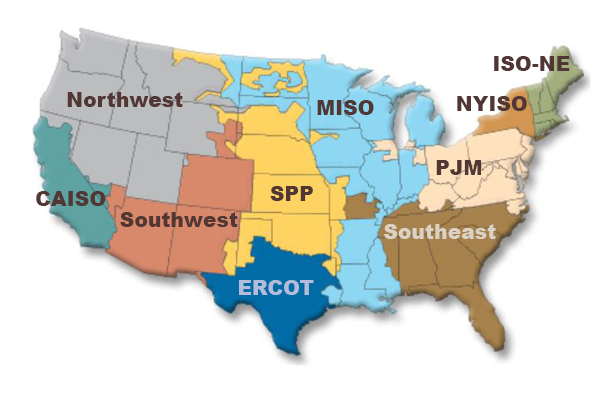
Read more information here:
Pandas and Energy Prices
The CSV (comma separated value) file Prices_DAM_ALTA2G_7_B1.csv contains price data for a single location in California for an entire year. The prices are set every hour and have units $/MWh. We will use the package pandas to import and analyze the data.
# Load the data file
ca_data = pd.read_csv("https://raw.githubusercontent.com/ndcbe/optimization/main/notebooks/data/Prices_DAM_ALTA2G_7_B1.csv", names=["price"])

# Print the first 10 rows
ca_data.head()Next we can calculate summary statistics:
ca_data.describe()Activity
What are 2 or 3 interesting observations from these summary statistics?Next, let’s visualize the data in a histogram:
plt.hist(ca_data["price"], color=BLUE)
plt.xlabel("Day-Ahead Market Energy Price [$/MWh]")
plt.ylabel("Count [hours in the year]")
plt.show()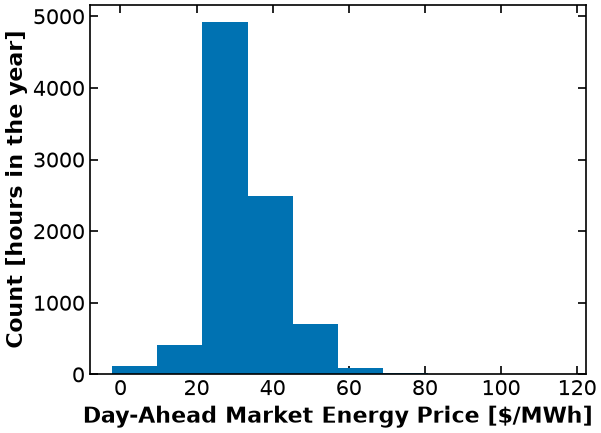
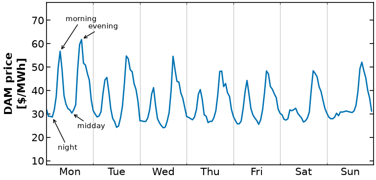
Finally, let’s visualize the prices during the first full calendar week. The data are for calendar year 2015. For reference, January 1, 2015 was a Thursday.
# ---------- EXTRACT --------------------------------------------------------
offset = 4  # days. January 1, 2015 was a Thursday, so +4 days lands on Monday.
number_of_days = 7
first_week = ca_data["price"].to_numpy()[
    (0 + offset) * 24 : (0 + offset + number_of_days) * 24
]

# The four features of the daily cycle worth naming, measured on the MONDAY of
# this window -- the day on which all four are cleanest. The same four recur
# every day; that is the point of showing seven.
feature_hours = {"night": 3, "morning": 7, "midday": 13, "evening": 18}
for label, hour in feature_hours.items():
    print(f"hour {hour:>2}   ${first_week[hour]:6.2f}/MWh   {label}")

results = {
    "price": first_week.tolist(),
    "n_days": number_of_days,
    "day_names": ["Mon", "Tue", "Wed", "Thu", "Fri", "Sat", "Sun"],
    "features": [{"label": k, "hour": v} for k, v in feature_hours.items()],
    "start": "2015-01-05",
}

# ---------- ARCHIVE --------------------------------------------------------
# figures/results/dam-price-week.json, committed to the repo. `source_tag` is
# None because there is no model to pin this to -- it is a DATA figure, and
# scripts/check_results_fresh.py reports it as UNVERIFIED rather than failing.
helper.save_results(
    "dam-price-week",
    results,
    notebook="notebooks/1-dev/Pyomo-Nuts-and-Bolts.ipynb",
    source_tag=None,
    description="One calendar week of CAISO day-ahead price at node "
    "ALTA2G_7_B1, Monday 5 to Sunday 11 January 2015, hourly.",
    solver=None,
);
hour 3 $ 28.66/MWh night
hour 7 $ 56.75/MWh morning
hour 13 $ 30.32/MWh midday
hour 18 $ 61.76/MWh evening
[helper] wrote figures/results/dam-price-week.json
# Tagged `figure:dam-price-week`: this cell is the single source of the figure
# in the Lecture 1 handout. See figures/README.md.
from matplotlib.ticker import MultipleLocator


def plot_dam_price_week(results):
    """One calendar week of day-ahead price: the cycle a battery is paid to exploit.

    CAISO day-ahead market, node ALTA2G_7_B1, calendar year 2015, hourly.
    January 1 2015 was a Thursday, so the `offset = 4` above starts the window
    on Monday, January 5 -- one full Monday-to-Sunday week.

    The four features are annotated on MONDAY ONLY. The same four recur every
    day of the week -- that is why seven days are shown -- but seven copies of
    four labels is noise, so the pattern is named once and left for the eye to
    repeat. The one-word labels are also the longest that fit: "morning peak"
    and "evening peak" collide at this aspect ratio, because the two features
    are 11 hours apart on a 168 hour axis.

    Greyscale: ONE series, and the annotations are black text with black
    arrows. The only other ink is the day grid, drawn as light rules rather
    than as a second series. Nothing here is keyed by colour.
    """
    week = np.array(results["price"])
    n_days = results["n_days"]
    day_names = results["day_names"]
    hours = np.arange(week.size)

    blue = "#0072B2"  # Okabe-Ito; the same blue the arbitrage figure uses

    # Text offsets in points, per feature. Set by looking at the rendered
    # figure, not guessed: all four sit inside Monday, only 15 hours apart on a
    # 168 hour axis, so the labels are STAGGERED vertically as well as offset
    # horizontally -- side by side they overlap.
    offsets = {
        "night": ((8, -40), "left", "top"),
        "morning": ((8, 42), "left", "bottom"),
        "midday": ((8, -14), "left", "top"),
        "evening": ((10, 14), "left", "bottom"),
    }

    fig, ax = plt.subplots(figsize=(8.0, 4.0))
    ax.plot(hours, week, linewidth=2.0, color=blue, linestyle="-")

    ax.xaxis.set_major_locator(MultipleLocator(24))
    ax.xaxis.set_minor_locator(MultipleLocator(6))
    for boundary in range(24, n_days * 24, 24):
        ax.axvline(boundary, color="0.75", linewidth=0.8, zorder=0)

    # Day names sit under the axis in place of a second set of tick labels:
    # "hour 96" means nothing, "Thu" means something.
    ax.set_xticks(24 * np.arange(n_days) + 12, minor=False)
    ax.set_xticklabels(day_names)
    ax.xaxis.set_minor_locator(MultipleLocator(24))
    ax.tick_params(axis="x", which="major", length=0)

    ax.set_xlim(0, n_days * 24)
    ax.set_ylabel("DAM price\n[\\$/MWh]")
    # No x-axis label: the day names already say what the window is, and the
    # caption carries the date.

    # Headroom above and below so the four labels clear the axes.
    lo, hi = week.min(), week.max()
    ax.set_ylim(lo - 0.42 * (hi - lo), hi + 0.42 * (hi - lo))

    # --- the four arrows --------------------------------------------------
    # An arrow is not a series: it gets no linestyle from the colour cycle, so
    # colour would be all it had. These are black, and each is labelled in
    # place with the feature it points at (figures/README.md).
    for feature in results["features"]:
        text = feature["label"]
        hour = feature["hour"]
        (dx, dy), ha, va = offsets[text]
        ax.annotate(
            text,
            xy=(hour, week[hour]),
            xytext=(dx, dy),
            textcoords="offset points",
            fontsize=11,
            ha=ha,
            va=va,
            color="black",
            linespacing=0.95,
            arrowprops=dict(
                arrowstyle="->",
                color="black",
                linewidth=1.1,
                shrinkA=1.0,
                shrinkB=3.0,
            ),
        )

    fig.tight_layout()
    return fig


fig = plot_dam_price_week(results)

# Write media/figures/dam-price-week.{png,pdf} -- what the Lecture 1 handout
# \includegraphics. A no-op on Colab, where there is no repo to write to.
helper.save_figure(fig, "dam-price-week");
[helper] wrote media/figures/dam-price-week.png and .pdf
Activity
What are 1 or 2 interesting observations from these plots?Optimization Mathematical Model
Energy (price) arbitrage is the idea of using energy storage (e.g., a battery) to take advantage of the significant daily energy price swings. This gives rise to many analysis questions including:
If a battery energy storage system perfectly timed its energy purchases and sales (i.e., it could perfectly forecast the market price), how much money could it make from energy arbitrage?
We can answer this question using mathematical/computational optimization!
Let’s start by drawing a picture.

Sets
Let’s say we want to define our optimization problem over a 24 hour window. The day-ahead market sets the energy prices in 1-hour intervals. We’ll define the set
for time where for a 24-hour planning horizon. For convenience, we’ll also define , which is the original set subtract subset .
Variables
Next, let’s identify the variables in the optimization problem:
, energy stored in battery at time , units: MWh
, battery discharge power (sold to market) during time interval [t-1, t), units: MW
, battery charge power (purchased from the market) during time interval [t-1, t), units: MW
Notice how all of these variables are indexed by the timestep . We’ll write in the model
Parameters
Parameters are data that are constant during the optimization problem. Here we have:
: Energy price during time interval [t-1, t), units: $/MWh
: Round trip efficiency, units: dimensionless
Maximum charge power, units: MW
Maximum discharge power, units: MW
Maximum storage energy, units: MWh
Energy in storage at time , units: MWh
hour, Timestep for grid decisions and prices (fixed)
Objective and Constraints
Finally, we’ll identify the objective, which is the function to improve, and the mathematical constraints. Below is the full mathematical model for the problem:
Activity
Write on paper a 1-sentence description for each equation.Degree of Freedom Analysis
Before we program our model in Pyomo, it is very important to first perform a degree of freedom analysis. Here are the steps:
Count the number of variables
Count the number of equality constraints
Degrees of freedom = number of variables subtract number of equality constraints
The degrees of freedom are the number of decision variables that can be freely manipulated by the optimizer. If there are no degrees of freedom, we often say the problem is square or it is a simulation problem.
For now, we will ignore inequality constraints and bounds. Later in the semester we will revisit degree of freedom analysis using some optimization theory concepts (e.g., active sets).
Activity
Perform degree of freedom analysis.Pyomo Modeling Components
Create ConcreteModel
We will start by creating a concrete Pyomo model. Recall, Pyomo is an object-oriented algebraic modeling language. The line below creates an instance of the ConcreteModel class.
m = pyo.ConcreteModel()For those unfamiliar with object-oriented programming, m is a container to define an optimization model. It includes a bunch of functionality to interface with different optimization solvers, perform diagnostics, and inspect the solution.
Pyomo also supports abstract models, but we will stick with concrete models this semester. See the Pyomo textbook for more details if you are curious.
Sets
We start by declaring a set for time. From above, recall we want to index all of the variables and constraints over the set
# Save the number of timesteps
m.N = 24

# Define the horizon set
m.HORIZON = pyo.Set(initialize=range(1, m.N + 1))
Some Pyomo modelers prefer to use all capital names for sets; this is a personal preference.
Variables
Next, we can declare our three variables: , ,
# Charging rate [MW]
m.c = pyo.Var(
    m.HORIZON, initialize=0.0, bounds=(0, 1), domain=pyo.NonNegativeReals, units=u.MW
)

# Discharging rate [MW]
m.d = pyo.Var(
    m.HORIZON, initialize=0.0, bounds=(0, 1), domain=pyo.NonNegativeReals, units=u.MW
)

# Energy (state-of-charge) [MWh]
m.E = pyo.Var(
    m.HORIZON, initialize=0.0, bounds=(0, 4), domain=pyo.NonNegativeReals, units=u.MWh
)
The keyword arguments for Var are collected below. Compiled from the
Pyomo documentation
and checked line by line against the Var constructor in Pyomo 6.10.1, the version this notebook runs on.
| Keyword | What it controls | Accepted values |
|---|---|---|
| (positional) | The index set(s). Each additional positional argument adds another index dimension, so pyo.Var(m.HORIZON, m.SCENARIOS) gives m.x[t, s]. | one or more Pyomo Set objects, or anything Pyomo can build a set from — a list, a range, a dict’s keys |
within or domain | The values the variable is allowed to take. This is also where integrality comes from: domain=pyo.Binary is what makes a variable binary. The two spellings are aliases — pass one, not both. | a virtual set (next table), any Pyomo Set, or a rule returning one. Default: Reals |
bounds | Lower and upper bound. | a (lower, upper) tuple, or a rule f(model, *index) returning one. None on either side means no bound on that side |
initialize or rule | The starting value the solver is handed. Matters a great deal for nonlinear models. Aliases — pass one, not both. | a scalar, a dict keyed by the index set, or a rule f(model, *index) |
units | Physical units, carried through every expression the variable appears in and checkable with assert_units_consistent. | a Pyomo units expression, e.g. u.MW |
dense | Whether a data object is built for every index at construction time (True) or only as indices are touched (False). | True (default) or False. Ignored, with a warning, on a scalar Var |
name, doc | Display name and documentation string. Cosmetic — they change pprint() output, not the model. | strings |
Notice the units= keyword. Pyomo carries units through every expression it builds, and
pyomo.util.check_units.assert_units_consistent then checks them. Declaring units and
never checking them is worse than not declaring them at all: it looks verified.
We call that check once the model is complete, further down.
The within/domain keyword takes a virtual set — a global object Pyomo predefines, which you
reference but never construct. Here is the full list, from the
Pyomo documentation
and cross-checked against the GlobalSets registry of the installed Pyomo 6.10.1.
| Virtual set | Members |
|---|---|
Any | anything at all, including None |
AnyWithNone | ⚠ deprecated since Pyomo 5.7 — use Any, which already admits None. Referencing it prints a deprecation warning |
EmptySet | nothing; no value is a member |
Reals | every real (floating point) number |
PositiveReals | reals strictly greater than zero, |
NonNegativeReals | reals greater than or equal to zero, |
NegativeReals | reals strictly less than zero, |
NonPositiveReals | reals less than or equal to zero, |
PercentFraction | reals in the closed interval |
UnitInterval | the same set as PercentFraction |
Integers | every whole number |
PositiveIntegers | whole numbers from 1 up |
NonNegativeIntegers | whole numbers from 0 up |
NegativeIntegers | whole numbers from -1 down |
NonPositiveIntegers | whole numbers from 0 down |
Binary | the two integers |
Boolean | the two integers — the same members as Binary |
Putting a variable in Integers, Binary, or any of the integer sets is what turns the problem into
an integer program. Ipopt handles continuous variables only and will refuse such a model; we switch
solvers for those, as we do at the end of this notebook.
In the example above, domain=pyo.NonNegativeReals is not needed, as we are specifying stricter bounds. It is included above to show the syntax.
Parameters (Constants / Data)
The next step is to define the parameter data: (energy prices), (round trip efficiency) and (intial energy storage level).
# Square root of round trip efficiency
m.sqrteta = pyo.Param(initialize=pyo.sqrt(0.88))

# Energy in battery at t=0
m.E0 = pyo.Param(initialize=2.0, mutable=True, units=u.MWh)

# Timestep for grid decisions and prices [hr]
m.dt = pyo.Param(initialize=1.0, units=u.hr)m.pprint()1 Set Declarations
HORIZON : Size=1, Index=None, Ordered=Insertion
Key : Dimen : Domain : Size : Members
None : 1 : Any : 24 : {1, 2, 3, 4, 5, 6, 7, 8, 9, 10, 11, 12, 13, 14, 15, 16, 17, 18, 19, 20, 21, 22, 23, 24}
3 Param Declarations
E0 : Size=1, Index=None, Domain=Any, Default=None, Mutable=True, Units=MWh
Key : Value
None : 2.0
dt : Size=1, Index=None, Domain=Any, Default=None, Mutable=True, Units=h
Key : Value
None : 1.0
sqrteta : Size=1, Index=None, Domain=Any, Default=None, Mutable=False
Key : Value
None : 0.938083151964686
3 Var Declarations
E : Size=24, Index=HORIZON, Units=MWh
Key : Lower : Value : Upper : Fixed : Stale : Domain
1 : 0 : 0.0 : 4 : False : False : NonNegativeReals
2 : 0 : 0.0 : 4 : False : False : NonNegativeReals
3 : 0 : 0.0 : 4 : False : False : NonNegativeReals
4 : 0 : 0.0 : 4 : False : False : NonNegativeReals
5 : 0 : 0.0 : 4 : False : False : NonNegativeReals
6 : 0 : 0.0 : 4 : False : False : NonNegativeReals
7 : 0 : 0.0 : 4 : False : False : NonNegativeReals
8 : 0 : 0.0 : 4 : False : False : NonNegativeReals
9 : 0 : 0.0 : 4 : False : False : NonNegativeReals
10 : 0 : 0.0 : 4 : False : False : NonNegativeReals
11 : 0 : 0.0 : 4 : False : False : NonNegativeReals
12 : 0 : 0.0 : 4 : False : False : NonNegativeReals
13 : 0 : 0.0 : 4 : False : False : NonNegativeReals
14 : 0 : 0.0 : 4 : False : False : NonNegativeReals
15 : 0 : 0.0 : 4 : False : False : NonNegativeReals
16 : 0 : 0.0 : 4 : False : False : NonNegativeReals
17 : 0 : 0.0 : 4 : False : False : NonNegativeReals
18 : 0 : 0.0 : 4 : False : False : NonNegativeReals
19 : 0 : 0.0 : 4 : False : False : NonNegativeReals
20 : 0 : 0.0 : 4 : False : False : NonNegativeReals
21 : 0 : 0.0 : 4 : False : False : NonNegativeReals
22 : 0 : 0.0 : 4 : False : False : NonNegativeReals
23 : 0 : 0.0 : 4 : False : False : NonNegativeReals
24 : 0 : 0.0 : 4 : False : False : NonNegativeReals
c : Size=24, Index=HORIZON, Units=MW
Key : Lower : Value : Upper : Fixed : Stale : Domain
1 : 0 : 0.0 : 1 : False : False : NonNegativeReals
2 : 0 : 0.0 : 1 : False : False : NonNegativeReals
3 : 0 : 0.0 : 1 : False : False : NonNegativeReals
4 : 0 : 0.0 : 1 : False : False : NonNegativeReals
5 : 0 : 0.0 : 1 : False : False : NonNegativeReals
6 : 0 : 0.0 : 1 : False : False : NonNegativeReals
7 : 0 : 0.0 : 1 : False : False : NonNegativeReals
8 : 0 : 0.0 : 1 : False : False : NonNegativeReals
9 : 0 : 0.0 : 1 : False : False : NonNegativeReals
10 : 0 : 0.0 : 1 : False : False : NonNegativeReals
11 : 0 : 0.0 : 1 : False : False : NonNegativeReals
12 : 0 : 0.0 : 1 : False : False : NonNegativeReals
13 : 0 : 0.0 : 1 : False : False : NonNegativeReals
14 : 0 : 0.0 : 1 : False : False : NonNegativeReals
15 : 0 : 0.0 : 1 : False : False : NonNegativeReals
16 : 0 : 0.0 : 1 : False : False : NonNegativeReals
17 : 0 : 0.0 : 1 : False : False : NonNegativeReals
18 : 0 : 0.0 : 1 : False : False : NonNegativeReals
19 : 0 : 0.0 : 1 : False : False : NonNegativeReals
20 : 0 : 0.0 : 1 : False : False : NonNegativeReals
21 : 0 : 0.0 : 1 : False : False : NonNegativeReals
22 : 0 : 0.0 : 1 : False : False : NonNegativeReals
23 : 0 : 0.0 : 1 : False : False : NonNegativeReals
24 : 0 : 0.0 : 1 : False : False : NonNegativeReals
d : Size=24, Index=HORIZON, Units=MW
Key : Lower : Value : Upper : Fixed : Stale : Domain
1 : 0 : 0.0 : 1 : False : False : NonNegativeReals
2 : 0 : 0.0 : 1 : False : False : NonNegativeReals
3 : 0 : 0.0 : 1 : False : False : NonNegativeReals
4 : 0 : 0.0 : 1 : False : False : NonNegativeReals
5 : 0 : 0.0 : 1 : False : False : NonNegativeReals
6 : 0 : 0.0 : 1 : False : False : NonNegativeReals
7 : 0 : 0.0 : 1 : False : False : NonNegativeReals
8 : 0 : 0.0 : 1 : False : False : NonNegativeReals
9 : 0 : 0.0 : 1 : False : False : NonNegativeReals
10 : 0 : 0.0 : 1 : False : False : NonNegativeReals
11 : 0 : 0.0 : 1 : False : False : NonNegativeReals
12 : 0 : 0.0 : 1 : False : False : NonNegativeReals
13 : 0 : 0.0 : 1 : False : False : NonNegativeReals
14 : 0 : 0.0 : 1 : False : False : NonNegativeReals
15 : 0 : 0.0 : 1 : False : False : NonNegativeReals
16 : 0 : 0.0 : 1 : False : False : NonNegativeReals
17 : 0 : 0.0 : 1 : False : False : NonNegativeReals
18 : 0 : 0.0 : 1 : False : False : NonNegativeReals
19 : 0 : 0.0 : 1 : False : False : NonNegativeReals
20 : 0 : 0.0 : 1 : False : False : NonNegativeReals
21 : 0 : 0.0 : 1 : False : False : NonNegativeReals
22 : 0 : 0.0 : 1 : False : False : NonNegativeReals
23 : 0 : 0.0 : 1 : False : False : NonNegativeReals
24 : 0 : 0.0 : 1 : False : False : NonNegativeReals
7 Declarations: HORIZON c d E sqrteta E0 dt
We see the initialize keyword is used to set the parameter value. When mutable=True, Pyomo builds
the model such that we can easily update the parameter and resolve. Later in the notebook, we will see
how this is helpful.
The keyword arguments for Param, from the
Pyomo documentation
and checked against the Param constructor in Pyomo 6.10.1:
| Keyword | What it controls | Accepted values |
|---|---|---|
| (positional) | The index set(s), exactly as for Var. | one or more Pyomo Set objects, or anything Pyomo can build a set from |
initialize or rule | The value(s). Aliases — pass one, not both. A dict is by far the most reliable form, because its keys must line up with the index set, and Pyomo will tell you when they do not. | a scalar, a dict keyed by the index set, or a rule f(model, *index) |
default | The value used for any index that initialize did not supply. Without it, reading an uninitialized index is an error. | a scalar, a dict, or a rule |
within or domain | The values the parameter is allowed to take; Pyomo rejects an initialization outside it. Default is Any, i.e. no restriction — note this differs from Var, whose default is Reals. | a virtual set, any Pyomo Set, or a rule returning one |
validate | A stricter check than domain: your own function, called once per value. Return False and construction fails with an error naming the index. | a callable f(model, value, *index) returning True/False |
mutable | Whether the value may be changed after construction and the model re-solved without rebuilding it. Default False. | True / False |
initialize_as_dense | Whether to build a data object for every index up front rather than lazily. | True / False (default) |
units | Physical units, carried into every expression the parameter appears in. | a Pyomo units expression, e.g. u.hr |
name, doc | Display name and documentation string. | strings |
Let’s dig in more to the initialize syntax. First, let’s convert the price data from pandas into a numpy array:
my_np_array = ca_data["price"].to_numpy()

# get the length
print("len(my_np_array) =", len(my_np_array))
len(my_np_array) = 8760
Recall, our dataset contains an entire year (which has 8760 hours). To access the first 24 hours, we use the following slice:
my_np_array[0:24]array([36.757, 34.924, 33.389, 32.035, 33.694, 36.88 , 38.662, 38.975,
35.08 , 29.979, 27.546, 25.944, 24.587, 23.788, 25.236, 30.145,
44.622, 50.957, 59.345, 52.564, 52.819, 48.816, 46.685, 38.575])len(my_np_array[0:24])24Initializing parameters in Pyomo can be precarious. The most fool proof strategy is to prepare a dictionary where the keys match the elements of the sets that index the parameter of interest. In our example, m.HORIZON contains 1, ..., 24, so we need a dictionary with the keys 1, ..., 24.
ca_data["price"][0:24].to_dict(){0: 36.757,
1: 34.924,
2: 33.389,
3: 32.035,
4: 33.694,
5: 36.88,
6: 38.662,
7: 38.975,
8: 35.08,
9: 29.979,
10: 27.546,
11: 25.944,
12: 24.587,
13: 23.788,
14: 25.236,
15: 30.145,
16: 44.622,
17: 50.957,
18: 59.345,
19: 52.564,
20: 52.819,
21: 48.816,
22: 46.685,
23: 38.575}That was easy. But what if we wanted to build the optimization model using the second day of data? Let’s give it a try:
ca_data["price"][24:48].to_dict(){24: 37.239,
25: 34.766,
26: 34.645,
27: 33.21,
28: 35.524,
29: 44.143,
30: 39.231,
31: 41.251,
32: 36.406,
33: 31.194,
34: 29.695,
35: 27.034,
36: 26.009,
37: 24.829,
38: 26.168,
39: 29.921,
40: 44.137,
41: 51.751,
42: 51.652,
43: 46.675,
44: 45.274,
45: 44.053,
46: 46.779,
47: 37.307}Activity
Uncomment the line below and look at the error message and read below. Then comment the line out again and rerun the notebook up to this cell.# DELIBERATE: this line is commented out on purpose, and stays that way.
# Uncomment it to trigger the KeyError explained in the next two cells, then
# comment it out again and re-run the notebook up to here. It is a teaching
# example of a Pyomo keying mistake, not dead code to be tidied away.
#
# m.price = pyo.Param(m.HORIZON, initialize=ca_data["price"][24:48].to_dict(), domain=pyo.Reals)You should get the following error:
ERROR: Constructing component 'price' from data=None failed: KeyError: "Index
    '25' is not valid for indexed component 'price'"
Why did this happen? Our dictionary is keyed 24 through 47, so it contains key 25, but we tried to create a Param indexed over 1 through 24.
Let’s say we want to build the optimization model starting for an arbitrary day. We need to extract the correct data from the pandas DataFrame and convert it to a dictionary with the correct keys. The function below does this using a simple, easy to follow approach. There is more compact “Pythonic” syntax to do this, but we will skip it for this getting started tutorial.
def prepare_price_data(day):
    """Prepare dictionary of price data

    Arguments:
        day: int, day to start. day = 0 is the first day

    Returns:
        data_dict: dictionary of price data with keys 1 to 24

    Notes:
        This function assumes the pandas DataFrame ca_data is in scope.

    """

    # Create empty dictionary
    data_dict = {}

    # Extract data as numpy array
    data_np_array = ca_data["price"][(day) * 24 : 24 * (day + 1)].to_numpy()

    # Loop over elements of numpy array
    for i in range(0, 24):

        # Add element to data_dict
        data_dict[i + 1] = data_np_array[i]

    return data_dict


# Create input data for day 1 (i.e., January 2, 2015)
my_data_dict = prepare_price_data(1)
print(my_data_dict)
{1: np.float64(37.239), 2: np.float64(34.766), 3: np.float64(34.645), 4: np.float64(33.21), 5: np.float64(35.524), 6: np.float64(44.143), 7: np.float64(39.231), 8: np.float64(41.251), 9: np.float64(36.406), 10: np.float64(31.194), 11: np.float64(29.695), 12: np.float64(27.034), 13: np.float64(26.009), 14: np.float64(24.829), 15: np.float64(26.168), 16: np.float64(29.921), 17: np.float64(44.137), 18: np.float64(51.751), 19: np.float64(51.652), 20: np.float64(46.675), 21: np.float64(45.274), 22: np.float64(44.053), 23: np.float64(46.779), 24: np.float64(37.307)}
Activity
Confirmmy_data_dict contains the correct prices for January 2, 2015.# Add your solution hereNow we are ready to define the price data parameter:
m.price = pyo.Param(
    m.HORIZON,
    initialize=my_data_dict,
    domain=pyo.Reals,
    mutable=True,
    units=u.USD / u.MWh,
)Objectives
Next, we will declare the objective function in Pyomo. Below are two equally valid syntaxes. The first, using the @m.Objective decorator, is the house style for this course. (The LP notebook has an aside comparing the decorator with the older rule= keyword; the two are equivalent.)
# Approach 1 (house style): the @m.Objective decorator
# Profit [USD] = price [USD/MWh] * dt [hr] * power [MW]
@m.Objective(sense=pyo.maximize)
def OBJ(b):
    return sum((-b.c[t] + b.d[t]) * b.price[t] * b.dt for t in b.HORIZON)


# Approach 2: build the expression inline with *expr=*
# m.OBJ = pyo.Objective(
#     expr=sum((-m.c[t] + m.d[t]) * m.price[t] * m.dt for t in m.HORIZON),
#     sense=pyo.maximize,
# )
Activity
Uncomment Approach 2 above and rerun the notebook. Pyomo will warn you it is replacing the componentOBJ, because Approach 1 already declared it. The answer should not change. Then comment Approach 2 out again.The keyword arguments for Objective, from the
Pyomo documentation
and checked against the Objective constructor in Pyomo 6.10.1:
| Keyword | What it controls | Accepted values |
|---|---|---|
| (positional) | The index set(s). An indexed Objective declares several objectives at once; a solver still needs exactly one of them active. | one or more Pyomo Set objects, or anything Pyomo can build a set from |
expr | The objective expression, written out directly. | any Pyomo expression |
rule | A function returning the objective expression. This is what the @m.Objective decorator above supplies. | a callable f(model, *index) returning a Pyomo expression, or Objective.Skip to declare nothing for that index |
sense | Minimize or maximize. Default: pyo.minimize. | pyo.minimize or pyo.maximize |
name, doc | Display name and documentation string. | strings |
Constraints
Now let’s add the last model component: the constraints.
# Define Energy Balance constraints. [MWh] = [MWh] + [hr]*[MW]
@m.Constraint(m.HORIZON)
def EnergyBalance_Con(b, t):
    # First timestep
    if t == 1:
        return b.E[t] == b.E0 + b.dt * (b.c[t] * b.sqrteta - b.d[t] / b.sqrteta)

    # Subsequent timesteps
    else:
        return b.E[t] == b.E[t - 1] + b.dt * (b.c[t] * b.sqrteta - b.d[t] / b.sqrteta)


# Periodic boundary: energy stored at the final time equals the initial [MWh]
m.PeriodicBoundaryCondition = pyo.Constraint(expr=m.E0 == m.E[m.N])

# The model is complete, so check the units.
# Raises UnitsError if any constraint or the objective is inconsistent.
assert_units_consistent(m)

print("Units are consistent.")
Units are consistent.
Notice what the timestep is doing here. The mathematical model on paper has it
in both the energy balance and the objective; the earlier version of this code dropped it,
because makes no numerical difference. Units are what make that
omission visible: without the energy balance sets MWh equal to MW, and
assert_units_consistent refuses it. Declaring the units restored the one-to-one
correspondence with the equations we wrote down.
That is the argument for units= over a comment. A comment such as
# [MWh] = [MW]*[1 hr] records the modeller’s intention; only the assertion checks that
the code did it.
We also see in this example a big advantage of defining a constraint with a rule
function instead of a single expr=. Inside the function EnergyBalance_Con we
incorporate a logical statement for how to handle the first timestep (which uses parameter
E0).
The keyword arguments for Constraint, from the
Pyomo documentation
and checked against the Constraint constructor in Pyomo 6.10.1:
| Keyword | What it controls | Accepted values |
|---|---|---|
| (positional) | The index set(s). One Constraint declaration then produces one constraint per index — which is how EnergyBalance_Con above becomes 24 rows. | one or more Pyomo Set objects, or anything Pyomo can build a set from |
expr | The constraint, written out directly. | a Pyomo expression containing a relational operator (==, <=, >=); a 2-tuple (value, body), which means equality; or a 3-tuple (lower, body, upper), a two-sided range |
rule | A function returning the constraint for each index. This is what the @m.Constraint(...) decorator above supplies, and it is what lets the first timestep be handled differently from the rest. | a callable f(model, *index) returning any of the forms in the row above, or Constraint.Skip to declare no constraint at that index |
name, doc | Display name and documentation string. | strings |
Activity
Compare the two model equations above to the optimization formulation below. Notice the one-to-one correspondence between the equality constraints in the mathematical formulation (below) and calls topyo.Constraint. Also notice the sets used to create the Pyomo model are listed next to each constraint in the mathematical model. Once you learn the Pyomo syntax, translating a mathematical model into code is easy!Printing the Model
Here is the optimization model, reproduced from above for convenience:
Now let’s see if our Pyomo model matches the optimization formulation. We will use the pprint() command (pretty print) to inspect the full model.
m.pprint()1 Set Declarations
HORIZON : Size=1, Index=None, Ordered=Insertion
Key : Dimen : Domain : Size : Members
None : 1 : Any : 24 : {1, 2, 3, 4, 5, 6, 7, 8, 9, 10, 11, 12, 13, 14, 15, 16, 17, 18, 19, 20, 21, 22, 23, 24}
4 Param Declarations
E0 : Size=1, Index=None, Domain=Any, Default=None, Mutable=True, Units=MWh
Key : Value
None : 2.0
dt : Size=1, Index=None, Domain=Any, Default=None, Mutable=True, Units=h
Key : Value
None : 1.0
price : Size=24, Index=HORIZON, Domain=Reals, Default=None, Mutable=True, Units=USD/MWh
Key : Value
1 : 37.239
2 : 34.766
3 : 34.645
4 : 33.21
5 : 35.524
6 : 44.143
7 : 39.231
8 : 41.251
9 : 36.406
10 : 31.194
11 : 29.695
12 : 27.034
13 : 26.009
14 : 24.829
15 : 26.168
16 : 29.921
17 : 44.137
18 : 51.751
19 : 51.652
20 : 46.675
21 : 45.274
22 : 44.053
23 : 46.779
24 : 37.307
sqrteta : Size=1, Index=None, Domain=Any, Default=None, Mutable=False
Key : Value
None : 0.938083151964686
3 Var Declarations
E : Size=24, Index=HORIZON, Units=MWh
Key : Lower : Value : Upper : Fixed : Stale : Domain
1 : 0 : 0.0 : 4 : False : False : NonNegativeReals
2 : 0 : 0.0 : 4 : False : False : NonNegativeReals
3 : 0 : 0.0 : 4 : False : False : NonNegativeReals
4 : 0 : 0.0 : 4 : False : False : NonNegativeReals
5 : 0 : 0.0 : 4 : False : False : NonNegativeReals
6 : 0 : 0.0 : 4 : False : False : NonNegativeReals
7 : 0 : 0.0 : 4 : False : False : NonNegativeReals
8 : 0 : 0.0 : 4 : False : False : NonNegativeReals
9 : 0 : 0.0 : 4 : False : False : NonNegativeReals
10 : 0 : 0.0 : 4 : False : False : NonNegativeReals
11 : 0 : 0.0 : 4 : False : False : NonNegativeReals
12 : 0 : 0.0 : 4 : False : False : NonNegativeReals
13 : 0 : 0.0 : 4 : False : False : NonNegativeReals
14 : 0 : 0.0 : 4 : False : False : NonNegativeReals
15 : 0 : 0.0 : 4 : False : False : NonNegativeReals
16 : 0 : 0.0 : 4 : False : False : NonNegativeReals
17 : 0 : 0.0 : 4 : False : False : NonNegativeReals
18 : 0 : 0.0 : 4 : False : False : NonNegativeReals
19 : 0 : 0.0 : 4 : False : False : NonNegativeReals
20 : 0 : 0.0 : 4 : False : False : NonNegativeReals
21 : 0 : 0.0 : 4 : False : False : NonNegativeReals
22 : 0 : 0.0 : 4 : False : False : NonNegativeReals
23 : 0 : 0.0 : 4 : False : False : NonNegativeReals
24 : 0 : 0.0 : 4 : False : False : NonNegativeReals
c : Size=24, Index=HORIZON, Units=MW
Key : Lower : Value : Upper : Fixed : Stale : Domain
1 : 0 : 0.0 : 1 : False : False : NonNegativeReals
2 : 0 : 0.0 : 1 : False : False : NonNegativeReals
3 : 0 : 0.0 : 1 : False : False : NonNegativeReals
4 : 0 : 0.0 : 1 : False : False : NonNegativeReals
5 : 0 : 0.0 : 1 : False : False : NonNegativeReals
6 : 0 : 0.0 : 1 : False : False : NonNegativeReals
7 : 0 : 0.0 : 1 : False : False : NonNegativeReals
8 : 0 : 0.0 : 1 : False : False : NonNegativeReals
9 : 0 : 0.0 : 1 : False : False : NonNegativeReals
10 : 0 : 0.0 : 1 : False : False : NonNegativeReals
11 : 0 : 0.0 : 1 : False : False : NonNegativeReals
12 : 0 : 0.0 : 1 : False : False : NonNegativeReals
13 : 0 : 0.0 : 1 : False : False : NonNegativeReals
14 : 0 : 0.0 : 1 : False : False : NonNegativeReals
15 : 0 : 0.0 : 1 : False : False : NonNegativeReals
16 : 0 : 0.0 : 1 : False : False : NonNegativeReals
17 : 0 : 0.0 : 1 : False : False : NonNegativeReals
18 : 0 : 0.0 : 1 : False : False : NonNegativeReals
19 : 0 : 0.0 : 1 : False : False : NonNegativeReals
20 : 0 : 0.0 : 1 : False : False : NonNegativeReals
21 : 0 : 0.0 : 1 : False : False : NonNegativeReals
22 : 0 : 0.0 : 1 : False : False : NonNegativeReals
23 : 0 : 0.0 : 1 : False : False : NonNegativeReals
24 : 0 : 0.0 : 1 : False : False : NonNegativeReals
d : Size=24, Index=HORIZON, Units=MW
Key : Lower : Value : Upper : Fixed : Stale : Domain
1 : 0 : 0.0 : 1 : False : False : NonNegativeReals
2 : 0 : 0.0 : 1 : False : False : NonNegativeReals
3 : 0 : 0.0 : 1 : False : False : NonNegativeReals
4 : 0 : 0.0 : 1 : False : False : NonNegativeReals
5 : 0 : 0.0 : 1 : False : False : NonNegativeReals
6 : 0 : 0.0 : 1 : False : False : NonNegativeReals
7 : 0 : 0.0 : 1 : False : False : NonNegativeReals
8 : 0 : 0.0 : 1 : False : False : NonNegativeReals
9 : 0 : 0.0 : 1 : False : False : NonNegativeReals
10 : 0 : 0.0 : 1 : False : False : NonNegativeReals
11 : 0 : 0.0 : 1 : False : False : NonNegativeReals
12 : 0 : 0.0 : 1 : False : False : NonNegativeReals
13 : 0 : 0.0 : 1 : False : False : NonNegativeReals
14 : 0 : 0.0 : 1 : False : False : NonNegativeReals
15 : 0 : 0.0 : 1 : False : False : NonNegativeReals
16 : 0 : 0.0 : 1 : False : False : NonNegativeReals
17 : 0 : 0.0 : 1 : False : False : NonNegativeReals
18 : 0 : 0.0 : 1 : False : False : NonNegativeReals
19 : 0 : 0.0 : 1 : False : False : NonNegativeReals
20 : 0 : 0.0 : 1 : False : False : NonNegativeReals
21 : 0 : 0.0 : 1 : False : False : NonNegativeReals
22 : 0 : 0.0 : 1 : False : False : NonNegativeReals
23 : 0 : 0.0 : 1 : False : False : NonNegativeReals
24 : 0 : 0.0 : 1 : False : False : NonNegativeReals
1 Objective Declarations
OBJ : Size=1, Index=None, Active=True
Key : Active : Sense : Expression
None : True : maximize : (- c[1] + d[1])*price[1]*dt + (- c[2] + d[2])*price[2]*dt + (- c[3] + d[3])*price[3]*dt + (- c[4] + d[4])*price[4]*dt + (- c[5] + d[5])*price[5]*dt + (- c[6] + d[6])*price[6]*dt + (- c[7] + d[7])*price[7]*dt + (- c[8] + d[8])*price[8]*dt + (- c[9] + d[9])*price[9]*dt + (- c[10] + d[10])*price[10]*dt + (- c[11] + d[11])*price[11]*dt + (- c[12] + d[12])*price[12]*dt + (- c[13] + d[13])*price[13]*dt + (- c[14] + d[14])*price[14]*dt + (- c[15] + d[15])*price[15]*dt + (- c[16] + d[16])*price[16]*dt + (- c[17] + d[17])*price[17]*dt + (- c[18] + d[18])*price[18]*dt + (- c[19] + d[19])*price[19]*dt + (- c[20] + d[20])*price[20]*dt + (- c[21] + d[21])*price[21]*dt + (- c[22] + d[22])*price[22]*dt + (- c[23] + d[23])*price[23]*dt + (- c[24] + d[24])*price[24]*dt
2 Constraint Declarations
EnergyBalance_Con : Size=24, Index=HORIZON, Active=True
Key : Lower : Body : Upper : Active
1 : 0.0 : E[1] - (E0 + dt*(0.938083151964686*c[1] - 1.0660035817780522*d[1])) : 0.0 : True
2 : 0.0 : E[2] - (E[1] + dt*(0.938083151964686*c[2] - 1.0660035817780522*d[2])) : 0.0 : True
3 : 0.0 : E[3] - (E[2] + dt*(0.938083151964686*c[3] - 1.0660035817780522*d[3])) : 0.0 : True
4 : 0.0 : E[4] - (E[3] + dt*(0.938083151964686*c[4] - 1.0660035817780522*d[4])) : 0.0 : True
5 : 0.0 : E[5] - (E[4] + dt*(0.938083151964686*c[5] - 1.0660035817780522*d[5])) : 0.0 : True
6 : 0.0 : E[6] - (E[5] + dt*(0.938083151964686*c[6] - 1.0660035817780522*d[6])) : 0.0 : True
7 : 0.0 : E[7] - (E[6] + dt*(0.938083151964686*c[7] - 1.0660035817780522*d[7])) : 0.0 : True
8 : 0.0 : E[8] - (E[7] + dt*(0.938083151964686*c[8] - 1.0660035817780522*d[8])) : 0.0 : True
9 : 0.0 : E[9] - (E[8] + dt*(0.938083151964686*c[9] - 1.0660035817780522*d[9])) : 0.0 : True
10 : 0.0 : E[10] - (E[9] + dt*(0.938083151964686*c[10] - 1.0660035817780522*d[10])) : 0.0 : True
11 : 0.0 : E[11] - (E[10] + dt*(0.938083151964686*c[11] - 1.0660035817780522*d[11])) : 0.0 : True
12 : 0.0 : E[12] - (E[11] + dt*(0.938083151964686*c[12] - 1.0660035817780522*d[12])) : 0.0 : True
13 : 0.0 : E[13] - (E[12] + dt*(0.938083151964686*c[13] - 1.0660035817780522*d[13])) : 0.0 : True
14 : 0.0 : E[14] - (E[13] + dt*(0.938083151964686*c[14] - 1.0660035817780522*d[14])) : 0.0 : True
15 : 0.0 : E[15] - (E[14] + dt*(0.938083151964686*c[15] - 1.0660035817780522*d[15])) : 0.0 : True
16 : 0.0 : E[16] - (E[15] + dt*(0.938083151964686*c[16] - 1.0660035817780522*d[16])) : 0.0 : True
17 : 0.0 : E[17] - (E[16] + dt*(0.938083151964686*c[17] - 1.0660035817780522*d[17])) : 0.0 : True
18 : 0.0 : E[18] - (E[17] + dt*(0.938083151964686*c[18] - 1.0660035817780522*d[18])) : 0.0 : True
19 : 0.0 : E[19] - (E[18] + dt*(0.938083151964686*c[19] - 1.0660035817780522*d[19])) : 0.0 : True
20 : 0.0 : E[20] - (E[19] + dt*(0.938083151964686*c[20] - 1.0660035817780522*d[20])) : 0.0 : True
21 : 0.0 : E[21] - (E[20] + dt*(0.938083151964686*c[21] - 1.0660035817780522*d[21])) : 0.0 : True
22 : 0.0 : E[22] - (E[21] + dt*(0.938083151964686*c[22] - 1.0660035817780522*d[22])) : 0.0 : True
23 : 0.0 : E[23] - (E[22] + dt*(0.938083151964686*c[23] - 1.0660035817780522*d[23])) : 0.0 : True
24 : 0.0 : E[24] - (E[23] + dt*(0.938083151964686*c[24] - 1.0660035817780522*d[24])) : 0.0 : True
PeriodicBoundaryCondition : Size=1, Index=None, Active=True
Key : Lower : Body : Upper : Active
None : E0 : E[24] : E0 : True
11 Declarations: HORIZON c d E sqrteta E0 dt price OBJ EnergyBalance_Con PeriodicBoundaryCondition
Activity
Does our Pyomo model match the optimization mathematical model (equations above)? How did we incorporate the inequality constraints into the Pyomo model?Another Approach: Build the Model in a Function
To emphasize the tutorial nature of this example, we build the model one piece at a time above. An often preferred approach is to define a Python function that builds the model, such as the one below.
Activity
The function below uses elements ofprice directly. Update the function to add the price data as a parameter in the Pyomo model. Make this parameter mutable as shown above.# Build the storage model of eq. (1-1) as a function of the price signal
def build_model(price, e0=0):
"""
Create optimization model for MPC
Arguments (inputs):
price: NumPy array with energy price timeseries
e0: initial value for energy storage level
Returns (outputs):
my_model: Pyomo optimization model
"""
# ConcreteModel: data are known now, so components are built immediately
my_model = pyo.ConcreteModel()
## Define Sets
# Number of timesteps in planning horizon
my_model.HORIZON = pyo.Set(initialize=range(len(price)))
## Define Parameters
# Square root of round trip efficiency
my_model.sqrteta = pyo.Param(initialize=pyo.sqrt(0.88))
# Energy in battery at t=0 [MWh]
my_model.E0 = pyo.Param(initialize=e0, mutable=True, units=u.MWh)
# Timestep for grid decisions and prices [hr]
my_model.dt = pyo.Param(initialize=1.0, units=u.hr)
## Define variables
# Charging rate [MW]
my_model.c = pyo.Var(my_model.HORIZON, initialize=0.0, bounds=(0, 1), units=u.MW)
# Discharging rate [MW]
my_model.d = pyo.Var(my_model.HORIZON, initialize=0.0, bounds=(0, 1), units=u.MW)
# Energy (state-of-charge) [MWh]
my_model.E = pyo.Var(my_model.HORIZON, initialize=0.0, bounds=(0, 4), units=u.MWh)
## Define constraints
# Define Energy Balance constraints. [MWh] = [MWh] + [hr]*[MW]
@my_model.Constraint(my_model.HORIZON)
def EnergyBalance_Con(b, t):
# First timestep
if t == 0:
return b.E[t] == b.E0 + b.dt * (b.c[t] * b.sqrteta - b.d[t] / b.sqrteta)
# Subsequent timesteps
else:
return b.E[t] == b.E[t - 1] + b.dt * (
b.c[t] * b.sqrteta - b.d[t] / b.sqrteta
)
# Periodic boundary: energy stored at the final time equals the initial [MWh]
my_model.PeriodicBoundaryCondition = pyo.Constraint(
expr=my_model.E0 == my_model.E[len(price) - 1]
)
## Define the objective function (profit) [USD]
# Receding horizon. price is a plain NumPy array here, so its units [USD/MWh]
# are attached inline rather than declared on a Param.
def objfun(model):
return sum(
(-model.c[t] + model.d[t]) * (price[t] * u.USD / u.MWh) * model.dt
for t in model.HORIZON
)
my_model.OBJ = pyo.Objective(rule=objfun, sense=pyo.maximize)
# Raises UnitsError if any constraint or the objective is inconsistent
assert_units_consistent(my_model)
return my_modelCalling Optimization Solver
Now that our Pyomo model is complete, we can numerically solve the model!
SolverFactory and Solver Options
Algebraic Modeling Languages, including Pyomo, allow us to define optimization problems in a general, solver agnostic way. This means we can quickly swap between solvers.
We will start by using Ipopt. First, we will create an instance of the SolverFactory:
# Specify the solver
solver = pyo.SolverFactory("ipopt")
Next we can specify options for ipopt such as setting the maximum number of iterations to 50:
solver.options["max_iter"] = 50Above solver is a SolverFactory object which includes the dictionary options used to set solver specific options.
Finally, we are ready to solve our model!
results = solver.solve(m, tee=True)
assert pyo.check_optimal_termination(results), (
    f"Solve failed: status={results.solver.status}, "
    f"termination={results.solver.termination_condition}"
)
Ipopt 3.14.19: max_iter=50
******************************************************************************
This program contains Ipopt, a library for large-scale nonlinear optimization.
Ipopt is released as open source code under the Eclipse Public License (EPL).
For more information visit https://github.com/coin-or/Ipopt
******************************************************************************
This is Ipopt version 3.14.19, running with linear solver MUMPS 5.8.2.
Number of nonzeros in equality constraint Jacobian...: 96
Number of nonzeros in inequality constraint Jacobian.: 0
Number of nonzeros in Lagrangian Hessian.............: 0
Total number of variables............................: 72
variables with only lower bounds: 0
variables with lower and upper bounds: 72
variables with only upper bounds: 0
Total number of equality constraints.................: 25
Total number of inequality constraints...............: 0
inequality constraints with only lower bounds: 0
inequality constraints with lower and upper bounds: 0
inequality constraints with only upper bounds: 0
iter objective inf_pr inf_du lg(mu) ||d|| lg(rg) alpha_du alpha_pr ls
0 1.4391990e-16 1.99e+00 9.90e+00 -1.0 0.00e+00 - 0.00e+00 0.00e+00 0
1 1.6802497e-01 1.96e+00 9.85e+00 -1.0 1.99e+00 - 5.21e-03 1.44e-02f 1
   2  2.1332988e+00 1.75e+00 9.89e+00  -1.0 1.96e+00    -  1.53e-02 1.09e-01f  1
   3  2.8652446e+00 1.35e+00 8.39e+00  -1.0 2.08e+00    -  1.09e-01 2.30e-01f  1
   4 -4.0482581e+00 1.01e+00 7.83e+00  -1.0 1.86e+00    -  6.95e-02 2.48e-01f  1
   5 -1.9676532e+01 8.93e-01 8.09e+00  -1.0 7.32e+00    -  6.32e-02 1.17e-01f  1
   6 -3.4249188e+01 7.76e-01 7.89e+00  -1.0 6.21e+00    -  7.33e-02 1.32e-01f  1
   7 -4.6657256e+01 6.62e-01 6.69e+00  -1.0 4.81e+00    -  1.52e-01 1.47e-01f  1
   8 -5.7915679e+01 5.23e-01 5.29e+00  -1.0 3.16e+00    -  2.06e-01 2.09e-01f  1
   9 -6.3119259e+01 3.85e-01 3.92e+00  -1.0 1.34e+00    -  2.30e-01 2.65e-01f  1
iter    objective    inf_pr   inf_du lg(mu)  ||d||  lg(rg) alpha_du alpha_pr  ls
  10 -6.3706910e+01 3.12e-02 6.94e+00  -1.0 1.08e+00    -  2.85e-01 9.19e-01f  1
  11 -6.5994667e+01 7.15e-03 3.17e+00  -1.0 6.93e-01    -  4.40e-01 7.71e-01f  1
  12 -6.6628205e+01 3.78e-03 7.49e-01  -1.0 9.35e-01    -  1.00e+00 4.72e-01f  1
  13 -6.9888933e+01 5.35e-04 1.10e-01  -1.7 2.22e-01    -  8.88e-01 8.58e-01f  1
  14 -7.1043057e+01 8.75e-05 1.55e-02  -2.5 2.18e-01    -  7.83e-01 8.36e-01f  1
  15 -7.1364922e+01 1.18e-05 3.85e-02  -3.8 2.82e-01    -  6.56e-01 8.65e-01f  1
  16 -7.1428935e+01 4.44e-16 7.22e-03  -3.8 5.71e-02    -  8.66e-01 1.00e+00f  1
  17 -7.1430287e+01 4.44e-16 7.11e-15  -3.8 8.19e-03    -  1.00e+00 1.00e+00f  1
  18 -7.1437864e+01 4.44e-16 6.96e-15  -5.7 1.65e-03    -  1.00e+00 1.00e+00f  1
  19 -7.1437961e+01 8.88e-16 8.30e-15  -8.6 2.85e-05    -  1.00e+00 1.00e+00f  1

Number of Iterations....: 19

                                   (scaled)                 (unscaled)
Objective...............:  -7.1437960657726151e+01   -7.1437960657726151e+01
Dual infeasibility......:   8.2967961385731204e-15    8.2967961385731204e-15
Constraint violation....:   8.8817841970012523e-16    8.8817841970012523e-16
Variable bound violation:   3.9759409986572791e-08    3.9759409986572791e-08
Complementarity.........:   3.2570995536791059e-09    3.2570995536791059e-09
Overall NLP error.......:   3.2570995536791059e-09    3.2570995536791059e-09


Number of objective function evaluations             = 20
Number of objective gradient evaluations             = 20
Number of equality constraint evaluations            = 20
Number of inequality constraint evaluations          = 0
Number of equality constraint Jacobian evaluations   = 20
Number of inequality constraint Jacobian evaluations = 0
Number of Lagrangian Hessian evaluations             = 19
Total seconds in IPOPT                               = 0.102

EXIT: Optimal Solution Found.
The keyword argument tee=True tells the solver to display its output to the screen.
Interpreting Ipopt Output - Verifying Degree of Freedom Analysis
Your Ipopt output should include the following:
Number of nonzeros in equality constraint Jacobian...:       96
Number of nonzeros in inequality constraint Jacobian.:        0
Number of nonzeros in Lagrangian Hessian.............:        0

Total number of variables............................:       72
                     variables with only lower bounds:        0
                variables with lower and upper bounds:       72
                     variables with only upper bounds:        0
Total number of equality constraints.................:       25
Total number of inequality constraints...............:        0
        inequality constraints with only lower bounds:        0
   inequality constraints with lower and upper bounds:        0
        inequality constraints with only upper bounds:        0
Activity
Compare this output to your degree of freedom analysis.Inspecting the Solution
We can inspect the entire model solution using pprint().
m.pprint()1 Set Declarations
HORIZON : Size=1, Index=None, Ordered=Insertion
Key : Dimen : Domain : Size : Members
None : 1 : Any : 24 : {1, 2, 3, 4, 5, 6, 7, 8, 9, 10, 11, 12, 13, 14, 15, 16, 17, 18, 19, 20, 21, 22, 23, 24}
4 Param Declarations
E0 : Size=1, Index=None, Domain=Any, Default=None, Mutable=True, Units=MWh
Key : Value
None : 2.0
dt : Size=1, Index=None, Domain=Any, Default=None, Mutable=True, Units=h
Key : Value
None : 1.0
price : Size=24, Index=HORIZON, Domain=Reals, Default=None, Mutable=True, Units=USD/MWh
Key : Value
1 : 37.239
2 : 34.766
3 : 34.645
4 : 33.21
5 : 35.524
6 : 44.143
7 : 39.231
8 : 41.251
9 : 36.406
10 : 31.194
11 : 29.695
12 : 27.034
13 : 26.009
14 : 24.829
15 : 26.168
16 : 29.921
17 : 44.137
18 : 51.751
19 : 51.652
20 : 46.675
21 : 45.274
22 : 44.053
23 : 46.779
24 : 37.307
sqrteta : Size=1, Index=None, Domain=Any, Default=None, Mutable=False
Key : Value
None : 0.938083151964686
3 Var Declarations
E : Size=24, Index=HORIZON, Units=MWh
Key : Lower : Value : Upper : Fixed : Stale : Domain
1 : 0 : 2.000000000804785 : 4 : False : False : NonNegativeReals
2 : 0 : 2.0000000112993037 : 4 : False : False : NonNegativeReals
3 : 0 : 2.0000000319069975 : 4 : False : False : NonNegativeReals
4 : 0 : 2.938083201679067 : 4 : False : False : NonNegativeReals
5 : 0 : 2.9380832045919867 : 4 : False : False : NonNegativeReals
6 : 0 : 1.8720796035614873 : 4 : False : False : NonNegativeReals
7 : 0 : 1.0660035914895196 : 4 : False : False : NonNegativeReals
8 : 0 : -8.655638723553363e-09 : 4 : False : False : NonNegativeReals
9 : 0 : -9.115005753876427e-09 : 4 : False : False : NonNegativeReals
10 : 0 : -6.181424950803798e-09 : 4 : False : False : NonNegativeReals
11 : 0 : 0.24766733414144607 : 4 : False : False : NonNegativeReals
12 : 0 : 1.1857505048666765 : 4 : False : False : NonNegativeReals
13 : 0 : 2.12383367588992 : 4 : False : False : NonNegativeReals
14 : 0 : 3.061916847113209 : 4 : False : False : NonNegativeReals
15 : 0 : 4.000000018100228 : 4 : False : False : NonNegativeReals
16 : 0 : 4.00000003975941 : 4 : False : False : NonNegativeReals
17 : 0 : 4.000000038635377 : 4 : False : False : NonNegativeReals
18 : 0 : 2.933996437576945 : 4 : False : False : NonNegativeReals
19 : 0 : 1.8679928365314515 : 4 : False : False : NonNegativeReals
20 : 0 : 1.8679928136956352 : 4 : False : False : NonNegativeReals
21 : 0 : 1.8679928137794752 : 4 : False : False : NonNegativeReals
22 : 0 : 1.867992814896921 : 4 : False : False : NonNegativeReals
23 : 0 : 1.061916828884662 : 4 : False : False : NonNegativeReals
24 : 0 : 2.0 : 4 : False : False : NonNegativeReals
c : Size=24, Index=HORIZON, Units=MW
Key : Lower : Value : Upper : Fixed : Stale : Domain
1 : 0 : -9.076328447621595e-09 : 1 : False : False : NonNegativeReals
2 : 0 : 4.6129851843523947e-10 : 1 : False : False : NonNegativeReals
3 : 0 : 1.122514944905246e-08 : 1 : False : False : NonNegativeReals
4 : 0 : 1.0000000080920235 : 1 : False : False : NonNegativeReals
5 : 0 : -7.490198166696666e-09 : 1 : False : False : NonNegativeReals
6 : 0 : -9.73946041078044e-09 : 1 : False : False : NonNegativeReals
7 : 0 : -9.467503770713836e-09 : 1 : False : False : NonNegativeReals
8 : 0 : -9.62738555755113e-09 : 1 : False : False : NonNegativeReals
9 : 0 : -9.290166798169277e-09 : 1 : False : False : NonNegativeReals
10 : 0 : -7.355527199353288e-09 : 1 : False : False : NonNegativeReals
11 : 0 : 0.2640142612132261 : 1 : False : False : NonNegativeReals
12 : 0 : 1.0000000090593126 : 1 : False : False : NonNegativeReals
13 : 0 : 1.0000000093207904 : 1 : False : False : NonNegativeReals
14 : 0 : 1.0000000094853687 : 1 : False : False : NonNegativeReals
15 : 0 : 1.00000000928996 : 1 : False : False : NonNegativeReals
16 : 0 : 1.2446343188330316e-08 : 1 : False : False : NonNegativeReals
17 : 0 : -9.455132910884623e-09 : 1 : False : False : NonNegativeReals
18 : 0 : -9.763089225431266e-09 : 1 : False : False : NonNegativeReals
19 : 0 : -9.76086851816158e-09 : 1 : False : False : NonNegativeReals
20 : 0 : -9.544553817218357e-09 : 1 : False : False : NonNegativeReals
21 : 0 : -9.38896262841655e-09 : 1 : False : False : NonNegativeReals
22 : 0 : -9.129905968825594e-09 : 1 : False : False : NonNegativeReals
23 : 0 : -9.553001939840134e-09 : 1 : False : False : NonNegativeReals
24 : 0 : 1.0000000093514616 : 1 : False : False : NonNegativeReals
d : Size=24, Index=HORIZON, Units=MW
Key : Lower : Value : Upper : Fixed : Stale : Domain
1 : 0 : -8.742124515838657e-09 : 1 : False : False : NonNegativeReals
2 : 0 : -9.438788399508391e-09 : 1 : False : False : NonNegativeReals
3 : 0 : -9.453598751691869e-09 : 1 : False : False : NonNegativeReals
4 : 0 : -9.583826216205655e-09 : 1 : False : False : NonNegativeReals
5 : 0 : -9.323934919922207e-09 : 1 : False : False : NonNegativeReals
6 : 0 : 1.0000000094896713 : 1 : False : False : NonNegativeReals
7 : 0 : 0.7561663177961923 : 1 : False : False : NonNegativeReals
8 : 0 : 1.0000000087577736 : 1 : False : False : NonNegativeReals
9 : 0 : -7.744422310674892e-09 : 1 : False : False : NonNegativeReals
10 : 0 : -9.224806661720392e-09 : 1 : False : False : NonNegativeReals
11 : 0 : -9.38115043785625e-09 : 1 : False : False : NonNegativeReals
12 : 0 : -9.626755519759847e-09 : 1 : False : False : NonNegativeReals
13 : 0 : -9.676216348762537e-09 : 1 : False : False : NonNegativeReals
14 : 0 : -9.719046740968002e-09 : 1 : False : False : NonNegativeReals
15 : 0 : -9.669365106869226e-09 : 1 : False : False : NonNegativeReals
16 : 0 : -9.365331800203448e-09 : 1 : False : False : NonNegativeReals
17 : 0 : -7.266080721118435e-09 : 1 : False : False : NonNegativeReals
18 : 0 : 1.000000009495081 : 1 : False : False : NonNegativeReals
19 : 0 : 1.0000000094848978 : 1 : False : False : NonNegativeReals
20 : 0 : 1.3022687125349388e-08 : 1 : False : False : NonNegativeReals
21 : 0 : -8.340935817994683e-09 : 1 : False : False : NonNegativeReals
22 : 0 : -9.082574214544385e-09 : 1 : False : False : NonNegativeReals
23 : 0 : 0.7561662932747802 : 1 : False : False : NonNegativeReals
24 : 0 : -9.735617830533423e-09 : 1 : False : False : NonNegativeReals
1 Objective Declarations
OBJ : Size=1, Index=None, Active=True
Key : Active : Sense : Expression
None : True : maximize : (- c[1] + d[1])*price[1]*dt + (- c[2] + d[2])*price[2]*dt + (- c[3] + d[3])*price[3]*dt + (- c[4] + d[4])*price[4]*dt + (- c[5] + d[5])*price[5]*dt + (- c[6] + d[6])*price[6]*dt + (- c[7] + d[7])*price[7]*dt + (- c[8] + d[8])*price[8]*dt + (- c[9] + d[9])*price[9]*dt + (- c[10] + d[10])*price[10]*dt + (- c[11] + d[11])*price[11]*dt + (- c[12] + d[12])*price[12]*dt + (- c[13] + d[13])*price[13]*dt + (- c[14] + d[14])*price[14]*dt + (- c[15] + d[15])*price[15]*dt + (- c[16] + d[16])*price[16]*dt + (- c[17] + d[17])*price[17]*dt + (- c[18] + d[18])*price[18]*dt + (- c[19] + d[19])*price[19]*dt + (- c[20] + d[20])*price[20]*dt + (- c[21] + d[21])*price[21]*dt + (- c[22] + d[22])*price[22]*dt + (- c[23] + d[23])*price[23]*dt + (- c[24] + d[24])*price[24]*dt
2 Constraint Declarations
EnergyBalance_Con : Size=24, Index=HORIZON, Active=True
Key : Lower : Body : Upper : Active
1 : 0.0 : E[1] - (E0 + dt*(0.938083151964686*c[1] - 1.0660035817780522*d[1])) : 0.0 : True
2 : 0.0 : E[2] - (E[1] + dt*(0.938083151964686*c[2] - 1.0660035817780522*d[2])) : 0.0 : True
3 : 0.0 : E[3] - (E[2] + dt*(0.938083151964686*c[3] - 1.0660035817780522*d[3])) : 0.0 : True
4 : 0.0 : E[4] - (E[3] + dt*(0.938083151964686*c[4] - 1.0660035817780522*d[4])) : 0.0 : True
5 : 0.0 : E[5] - (E[4] + dt*(0.938083151964686*c[5] - 1.0660035817780522*d[5])) : 0.0 : True
6 : 0.0 : E[6] - (E[5] + dt*(0.938083151964686*c[6] - 1.0660035817780522*d[6])) : 0.0 : True
7 : 0.0 : E[7] - (E[6] + dt*(0.938083151964686*c[7] - 1.0660035817780522*d[7])) : 0.0 : True
8 : 0.0 : E[8] - (E[7] + dt*(0.938083151964686*c[8] - 1.0660035817780522*d[8])) : 0.0 : True
9 : 0.0 : E[9] - (E[8] + dt*(0.938083151964686*c[9] - 1.0660035817780522*d[9])) : 0.0 : True
10 : 0.0 : E[10] - (E[9] + dt*(0.938083151964686*c[10] - 1.0660035817780522*d[10])) : 0.0 : True
11 : 0.0 : E[11] - (E[10] + dt*(0.938083151964686*c[11] - 1.0660035817780522*d[11])) : 0.0 : True
12 : 0.0 : E[12] - (E[11] + dt*(0.938083151964686*c[12] - 1.0660035817780522*d[12])) : 0.0 : True
13 : 0.0 : E[13] - (E[12] + dt*(0.938083151964686*c[13] - 1.0660035817780522*d[13])) : 0.0 : True
14 : 0.0 : E[14] - (E[13] + dt*(0.938083151964686*c[14] - 1.0660035817780522*d[14])) : 0.0 : True
15 : 0.0 : E[15] - (E[14] + dt*(0.938083151964686*c[15] - 1.0660035817780522*d[15])) : 0.0 : True
16 : 0.0 : E[16] - (E[15] + dt*(0.938083151964686*c[16] - 1.0660035817780522*d[16])) : 0.0 : True
17 : 0.0 : E[17] - (E[16] + dt*(0.938083151964686*c[17] - 1.0660035817780522*d[17])) : 0.0 : True
18 : 0.0 : E[18] - (E[17] + dt*(0.938083151964686*c[18] - 1.0660035817780522*d[18])) : 0.0 : True
19 : 0.0 : E[19] - (E[18] + dt*(0.938083151964686*c[19] - 1.0660035817780522*d[19])) : 0.0 : True
20 : 0.0 : E[20] - (E[19] + dt*(0.938083151964686*c[20] - 1.0660035817780522*d[20])) : 0.0 : True
21 : 0.0 : E[21] - (E[20] + dt*(0.938083151964686*c[21] - 1.0660035817780522*d[21])) : 0.0 : True
22 : 0.0 : E[22] - (E[21] + dt*(0.938083151964686*c[22] - 1.0660035817780522*d[22])) : 0.0 : True
23 : 0.0 : E[23] - (E[22] + dt*(0.938083151964686*c[23] - 1.0660035817780522*d[23])) : 0.0 : True
24 : 0.0 : E[24] - (E[23] + dt*(0.938083151964686*c[24] - 1.0660035817780522*d[24])) : 0.0 : True
PeriodicBoundaryCondition : Size=1, Index=None, Active=True
Key : Lower : Body : Upper : Active
None : E0 : E[24] : E0 : True
11 Declarations: HORIZON c d E sqrteta E0 dt price OBJ EnergyBalance_Con PeriodicBoundaryCondition
The solution is stored in the value column. This is helpful for debugging small models but tedious otherwise.
Extracting Solution from Pyomo
A key advantage of Pyomo is that it is an Algebraic Modeling Language in Python. So let’s use Python to analyze the solution! The code below extracts the values of the variables into three lists.
# Declare empty lists
c_control = []
d_control = []
E_control = []
t = []

# Loop over elements of HORIZON set.
for i in m.HORIZON:

    t.append(pyo.value(i))

    # Use value( ) function to extract the solution for each variable and append to the results lists
    c_control.append(pyo.value(m.c[i]))

    # Adding negative sign to discharge for plotting
    d_control.append(-pyo.value(m.d[i]))
E_control.append(pyo.value(m.E[i]))print(c_control)[-9.076328447621595e-09, 4.6129851843523947e-10, 1.122514944905246e-08, 1.0000000080920235, -7.490198166696666e-09, -9.73946041078044e-09, -9.467503770713836e-09, -9.62738555755113e-09, -9.290166798169277e-09, -7.355527199353288e-09, 0.2640142612132261, 1.0000000090593126, 1.0000000093207904, 1.0000000094853687, 1.00000000928996, 1.2446343188330316e-08, -9.455132910884623e-09, -9.763089225431266e-09, -9.76086851816158e-09, -9.544553817218357e-09, -9.38896262841655e-09, -9.129905968825594e-09, -9.553001939840134e-09, 1.0000000093514616]
print(d_control)[8.742124515838657e-09, 9.438788399508391e-09, 9.453598751691869e-09, 9.583826216205655e-09, 9.323934919922207e-09, -1.0000000094896713, -0.7561663177961923, -1.0000000087577736, 7.744422310674892e-09, 9.224806661720392e-09, 9.38115043785625e-09, 9.626755519759847e-09, 9.676216348762537e-09, 9.719046740968002e-09, 9.669365106869226e-09, 9.365331800203448e-09, 7.266080721118435e-09, -1.000000009495081, -1.0000000094848978, -1.3022687125349388e-08, 8.340935817994683e-09, 9.082574214544385e-09, -0.7561662932747802, 9.735617830533423e-09]
print(E_control)[2.000000000804785, 2.0000000112993037, 2.0000000319069975, 2.938083201679067, 2.9380832045919867, 1.8720796035614873, 1.0660035914895196, -8.655638723553363e-09, -9.115005753876427e-09, -6.181424950803798e-09, 0.24766733414144607, 1.1857505048666765, 2.12383367588992, 3.061916847113209, 4.000000018100228, 4.00000003975941, 4.000000038635377, 2.933996437576945, 1.8679928365314515, 1.8679928136956352, 1.8679928137794752, 1.867992814896921, 1.061916828884662, 2.0]
Visualizing the Solution
You can debug the plot without re-solving. Getting three panels aligned and the labels off each other takes a dozen attempts. Each one should cost milliseconds, not another call to Ipopt.
You can archive the answer. Store the extracted results next to your paper and you can redraw the figure a year later, on a machine with no solver installed, from the numbers you actually reported.
In research code, pickle is the quick way to store them, and that is what I tell my students to reach for. Here the archive is committed to the repository, so it is written as JSON instead: a pickle in version control is an unreviewable binary that stops loading the next time a library is upgraded, and nobody can read its diff.
The three cells below are the single source of the figure that appears in the Lecture 1 handout --- there is no second script re-deriving this schedule somewhere else.
# ---------- SOLVE ----------------------------------------------------------
# The same 24 hour problem as above, built by the `build_model` function so the
# figure and the handout listing cannot drift apart. Nothing is plotted here.
price_day1 = ca_data["price"][24:48].to_numpy()
m_fig = build_model(price=price_day1, e0=2.0)

res_fig = solver.solve(m_fig)
assert pyo.check_optimal_termination(res_fig), "Solve failed"

# Same model, same answer as the piecewise build above.
assert abs(pyo.value(m_fig.OBJ) - pyo.value(m.OBJ)) < 1e-4

print(f"Optimal profit: ${pyo.value(m_fig.OBJ):,.2f} per day")
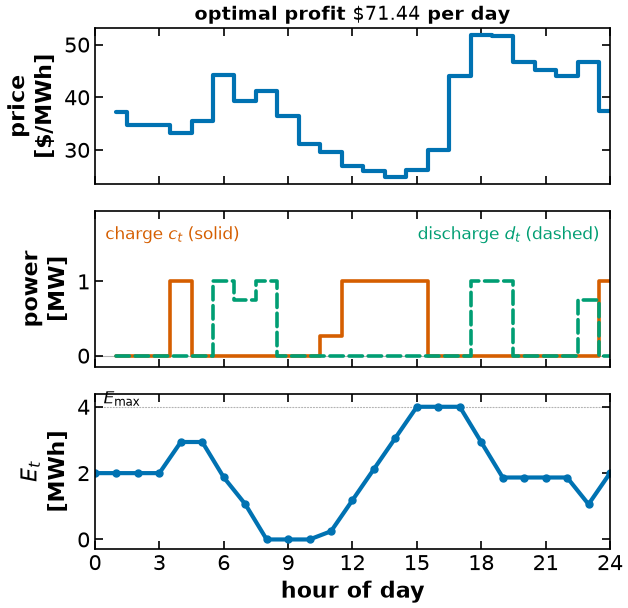
Optimal profit: $71.44 per day
# ---------- EXTRACT --------------------------------------------------------
# Pyomo objects -> plain Python. After this cell nothing below touches a model,
# a solver, or the raw price file.
results = {
    "price": [float(price_day1[t]) for t in m_fig.HORIZON],
    "charge": [pyo.value(m_fig.c[t]) for t in m_fig.HORIZON],
    "discharge": [pyo.value(m_fig.d[t]) for t in m_fig.HORIZON],
    "energy": [pyo.value(m_fig.E[t]) for t in m_fig.HORIZON],
    "profit": pyo.value(m_fig.OBJ),
    "E0": pyo.value(m_fig.E0),
    "E_max": m_fig.E[0].ub,
    "day": 1,
}

# The periodic boundary condition, checked on the extracted numbers rather than
# assumed: the battery ends the day exactly where it started.
assert abs(results["energy"][-1] - results["E0"]) < 1e-6

# ---------- ARCHIVE --------------------------------------------------------
# figures/results/battery-arbitrage.json, committed to the repo, so a change to
# the house STYLE can re-render this figure with no solver. `source_tag` points
# at the `build_model` cell above, so scripts/check_results_fresh.py can tell
# you when the model has changed and these numbers have not.
helper.save_results(
    "battery-arbitrage",
    results,
    notebook="notebooks/1-dev/Pyomo-Nuts-and-Bolts.ipynb",
    source_tag="handout:battery-model",
    description="Optimal energy arbitrage for a 24 h battery on CAISO day 1 "
    "(2 January 2015): price, the charge/discharge decision, and the state of "
    "charge.",
    solver="Ipopt via Pyomo",
);
[helper] wrote figures/results/battery-arbitrage.json
# The PLOTTING function: it reads the extracted results, not the Pyomo model.
#
# Everything it needs is in `results`, and nothing else -- no model, no solver,
# no data file. That is what lets you re-run this one cell as many times as it
# takes to get the panels lined up, without waiting for another solve.
#
# Tagged `figure:battery-arbitrage`, which makes this cell the single source of
# the figure in the Lecture 1 handout. See figures/README.md.


def plot_battery_arbitrage(results):
    """Price, the charge/discharge decision, and the state of charge.

    ONE three-panel figure, because the argument is the ALIGNMENT between the
    panels: the battery charges through the overnight trough, discharges into
    the two price peaks, and the state of charge is the running integral of
    what it did. Printing any panel on its own loses that.

    Colour: blue for price and for the state of charge, vermillion for
    charging, bluish green for discharging. Those are the Okabe-Ito members of
    the red and green hue families; matplotlib's bare 'r' and 'g' are the one
    pair a red-green colour-blind reader cannot separate at all. Vermillion
    (L* = 54.2) and bluish green (L* = 57.7) collapse to the SAME grey on a
    photocopier, so charging and discharging also differ in linestyle. Colour
    is never the only channel -- see figures/README.md.
    """
    price = np.array(results["price"])
    charge = np.array(results["charge"])
    discharge = np.array(results["discharge"])
    energy = np.array(results["energy"])
    e0 = results["E0"]
    e_max = results["E_max"]
    profit = results["profit"]
    n = price.size

    blue = "#0072B2"  # price, and state of charge
    vermillion = "#D55E00"  # charging   (buying from the market)
    bluish_green = "#009E73"  # discharging (selling to the market)

    hours = np.arange(1, n + 1)
    fig, axes = plt.subplots(3, 1, figsize=(6.6, 6.4), sharex=True)
    ax_p, ax_u, ax_e = axes

    # --- panel 1: the data ------------------------------------------------
    ax_p.step(hours, price, where="mid", color=blue, linestyle="-")
    ax_p.set_ylabel("price\n[\\$/MWh]")

    # --- panel 2: the decision --------------------------------------------
    ax_u.step(
        hours, charge, where="mid", color=vermillion, linestyle="-", linewidth=2.6
    )
    ax_u.step(
        hours, discharge, where="mid", color=bluish_green, linestyle="--", linewidth=2.6
    )
    ax_u.axhline(0.0, color="0.7", linewidth=0.8, zorder=0)
    ax_u.set_ylabel("power\n[MW]")
    ax_u.set_ylim(-0.15, 1.95)

    # Direct labelling, in the series colour -- preferred over a legend
    # (figures/README.md). Pinned in axes coordinates rather than to a data
    # point: c_t and d_t both max out at 1 MW, and the two labels landed on top
    # of each other when placed at their argmax.
    ax_u.annotate(
        "charge $c_t$ (solid)",
        xy=(0.02, 0.90),
        xycoords="axes fraction",
        color=vermillion,
        fontsize=12,
        ha="left",
        va="top",
    )
    ax_u.annotate(
        "discharge $d_t$ (dashed)",
        xy=(0.98, 0.90),
        xycoords="axes fraction",
        color=bluish_green,
        fontsize=12,
        ha="right",
        va="top",
    )

    # --- panel 3: the state -----------------------------------------------
    # NOT a step plot: energy is the integral of power, so E_t is piecewise
    # LINEAR in time. That is the modelling lesson this panel exists to make.
    ax_e.plot(
        np.concatenate([[0], hours]),
        np.concatenate([[e0], energy]),
        marker="o",
        markersize=5,
        color=blue,
        linestyle="-",
    )
    ax_e.set_ylabel("$E_t$\n[MWh]")
    ax_e.set_ylim(-0.3, e_max + 0.4)
    ax_e.axhline(e_max, color="0.7", linewidth=0.8, linestyle=":", zorder=0)
    ax_e.annotate("$E_{\\max}$", xy=(0.4, e_max + 0.08), fontsize=12)

    ax_e.set_xlabel("hour of day")
    ax_e.set_xlim(0, n)
    ax_e.set_xticks(range(0, 25, 3))

    ax_p.set_title(f"optimal profit $\\${profit:,.2f}$ per day", fontsize=14)

    fig.tight_layout()
    return fig


fig = plot_battery_arbitrage(results)

# Write media/figures/battery-arbitrage.{png,pdf} -- what the Lecture 1 handout
# \includegraphics. A no-op on Colab, where there is no repo to write to.
helper.save_figure(fig, "battery-arbitrage");
[helper] wrote media/figures/battery-arbitrage.png and .pdf
Accessing Dual Variables
### Declare all suffixes
# https://pyomo.readthedocs.io/en/stable/explanation/modeling/math_programming/suffixes.html#importing-suffix-data

# Ipopt bound multipliers
m.ipopt_zL_out = pyo.Suffix(direction=pyo.Suffix.IMPORT)
m.ipopt_zU_out = pyo.Suffix(direction=pyo.Suffix.IMPORT)

# Ipopt constraint multipliers
m.dual = pyo.Suffix(direction=pyo.Suffix.IMPORT_EXPORT)

# Resolve the model
results = solver.solve(m, tee=True)
assert pyo.check_optimal_termination(results), (
    f"Solve failed: status={results.solver.status}, "
    f"termination={results.solver.termination_condition}"
)
Ipopt 3.14.19: max_iter=50
******************************************************************************
This program contains Ipopt, a library for large-scale nonlinear optimization.
Ipopt is released as open source code under the Eclipse Public License (EPL).
For more information visit https://github.com/coin-or/Ipopt
******************************************************************************
This is Ipopt version 3.14.19, running with linear solver MUMPS 5.8.2.
Number of nonzeros in equality constraint Jacobian...: 96
Number of nonzeros in inequality constraint Jacobian.: 0
Number of nonzeros in Lagrangian Hessian.............: 0
Total number of variables............................: 72
variables with only lower bounds: 0
variables with lower and upper bounds: 72
variables with only upper bounds: 0
Total number of equality constraints.................: 25
Total number of inequality constraints...............: 0
inequality constraints with only lower bounds: 0
inequality constraints with lower and upper bounds: 0
inequality constraints with only upper bounds: 0
iter objective inf_pr inf_du lg(mu) ||d|| lg(rg) alpha_du alpha_pr ls
0 -7.0590011e+01 2.00e-02 9.90e+00 -1.0 0.00e+00 - 0.00e+00 0.00e+00 0
1 -6.7757766e+01 1.19e-02 6.76e+00 -1.0 2.29e-01 - 2.29e-01 4.04e-01f 1
2 -6.6680579e+01 4.44e-16 2.66e+00 -1.0 1.52e-01 - 7.71e-01 1.00e+00h 1
3 -6.6663394e+01 4.44e-16 7.55e-15 -1.0 8.79e-02 - 1.00e+00 1.00e+00f 1
4 -7.0905011e+01 4.44e-16 8.57e-03 -2.5 1.20e-01 - 9.06e-01 9.26e-01f 1
5 -7.1259816e+01 4.44e-16 8.80e-02 -2.5 1.57e-01 - 8.04e-01 1.00e+00f 1
6 -7.1294102e+01 4.44e-16 8.38e-15 -2.5 8.18e-02 - 1.00e+00 1.00e+00f 1
7 -7.1429428e+01 4.44e-16 8.69e-04 -3.8 2.94e-02 - 9.56e-01 1.00e+00f 1
8 -7.1437868e+01 4.44e-16 7.99e-15 -5.7 4.53e-03 - 1.00e+00 1.00e+00f 1
9 -7.1437961e+01 8.88e-16 7.48e-15 -8.6 2.04e-05 - 1.00e+00 1.00e+00f 1
Number of Iterations....: 9
(scaled) (unscaled)
Objective...............: -7.1437960657845522e+01 -7.1437960657845522e+01
Dual infeasibility......: 7.4779217428591052e-15 7.4779217428591052e-15
Constraint violation....: 8.8817841970012523e-16 8.8817841970012523e-16
Variable bound violation: 3.9759201264644162e-08 3.9759201264644162e-08
Complementarity.........: 3.3122665150541337e-09 3.3122665150541337e-09
Overall NLP error.......: 3.3122665150541337e-09 3.3122665150541337e-09
Number of objective function evaluations = 10
Number of objective gradient evaluations = 10
Number of equality constraint evaluations = 10
Number of inequality constraint evaluations = 0
Number of equality constraint Jacobian evaluations = 10
Number of inequality constraint Jacobian evaluations = 0
Number of Lagrangian Hessian evaluations = 9
Total seconds in IPOPT = 0.040
EXIT: Optimal Solution Found.
# Inspect dual variables for lower bound
m.ipopt_zL_out.display()
ipopt_zL_out : Direction=IMPORT, Datatype=FLOAT
Key : Value
E[10] : -0.794241619316072
E[11] : -9.959159559145174e-09
E[12] : -2.102627169661387e-09
E[13] : -1.175782908727664e-09
E[14] : -8.162117659813141e-10
E[15] : -6.2506885965562e-10
E[16] : -6.264563243789251e-10
E[17] : -6.263268931807182e-10
E[18] : -8.539379352204578e-10
E[19] : -1.341422206806913e-09
E[1] : -1.2527829785585504e-09
E[20] : -1.341350289904925e-09
E[21] : -1.3409814411365547e-09
E[22] : -1.3409540074980453e-09
E[23] : -2.3608437770291847e-09
E[24] : -1.2529517735752844e-09
E[2] : -1.2561427947619423e-09
E[3] : -1.2655652532929373e-09
E[4] : -8.577658488886522e-10
E[5] : -8.581114250870307e-10
E[6] : -1.3533628470961722e-09
E[7] : -2.3510746270035887e-09
E[8] : -1.2933647690071222
E[9] : -3.0593573861032906
c[10] : -0.7539353271121387
c[11] : -9.178573911933398e-09
c[12] : -2.5046223507521217e-09
c[13] : -2.504981145674995e-09
c[14] : -2.505204613811326e-09
c[15] : -2.5049335000765823e-09
c[16] : -0.09378257453432326
c[17] : -4.225625753907411
c[18] : -10.585480009504597
c[19] : -10.486480008099354
c[1] : -2.7157200105877193
c[20] : -5.509480008254767
c[21] : -4.1084800084101225
c[22] : -2.8874800085646593
c[23] : -5.613480008720141
c[24] : -2.505054971752294e-09
c[2] : -0.24272001057702478
c[3] : -0.1217200105783847
c[4] : -2.5032939579251872e-09
c[5] : -1.0007200092145052
c[6] : -9.619720007824004
c[7] : -4.707720007994102
c[8] : -6.7277200093986425
c[9] : -3.096003707960806
d[10] : -3.396982588174682
d[11] : -4.049318177854258
d[12] : -6.71031816795165
d[13] : -7.7353181666628466
d[14] : -8.915318166841939
d[15] : -7.576318168864481
d[16] : -3.9735652615436816
d[17] : -1.216834375909733
d[18] : -2.505198045055362e-09
d[19] : -2.5051853989409155e-09
d[1] : -1.9919999933188999
d[20] : -0.10399999597165342
d[21] : -1.50499999579355
d[22] : -2.7259999956183774
d[23] : -3.310230595020828e-09
d[24] : -9.471999993835604
d[2] : -4.464999993320209
d[3] : -4.585999993313965
d[4] : -6.020999993293633
d[5] : -3.706999994877842
d[6] : -2.5052181084524623e-09
d[7] : -3.4362028761281816e-09
d[8] : -2.504243095823582e-09
d[9] : -1.4462685190308162
# Inspect dual variables for upper bound
m.ipopt_zU_out.display()
ipopt_zU_out : Direction=IMPORT, Datatype=FLOAT
Key : Value
E[10] : 6.262126510435488e-10
E[11] : 6.693766261750669e-10
E[12] : 8.9355974571478e-10
E[13] : 1.3437267429111052e-09
E[14] : 2.713588361024654e-09
E[15] : 0.14094426689949266
E[16] : 10.74974729064419
E[17] : 1.336923856231947
E[18] : 2.351928363328083e-09
E[19] : 1.1754291485433243e-09
E[1] : 1.253120766471938e-09
E[20] : 1.175503900129797e-09
E[21] : 1.1758414697720055e-09
E[22] : 1.1758669537676752e-09
E[23] : 8.52768230140698e-10
E[24] : 1.2529517547809998e-09
E[2] : 1.2502665613514982e-09
E[3] : 1.24632281279438e-09
E[4] : 2.3442194466299494e-09
E[5] : 2.3435146974157423e-09
E[6] : 1.1716539589773153e-09
E[7] : 8.540487163434175e-10
E[8] : 6.263114689358477e-10
E[9] : 6.264067093301249e-10
c[10] : 2.501551046300082e-09
c[11] : 3.485865653996596e-09
c[12] : 2.660999988097329
c[13] : 3.685999986963479
c[14] : 4.865999987121249
c[15] : 3.526999988900875
c[16] : 2.488326784154284e-09
c[17] : 2.505087869933442e-09
c[18] : 2.5055784824939886e-09
c[19] : 2.505575764231218e-09
c[1] : 2.504663438587999e-09
c[20] : 2.5052724774879727e-09
c[21] : 2.5050505672851535e-09
c[22] : 2.5046738348391535e-09
c[23] : 2.5052848589351162e-09
c[24] : 3.8585199948754973
c[2] : 2.4942907974796294e-09
c[3] : 2.4901294446298907e-09
c[4] : 1.313279994396989
c[5] : 2.502622398305555e-09
c[6] : 2.50555189696077e-09
c[7] : 2.5051873502835386e-09
c[8] : 2.505400368423204e-09
c[9] : 2.504812685816175e-09
d[10] : 2.5048969816613713e-09
d[11] : 2.5050580104567345e-09
d[12] : 2.5053966054632424e-09
d[13] : 2.5054642903322925e-09
d[14] : 2.5055223105939546e-09
d[15] : 2.5054535422253457e-09
d[16] : 2.505042743787309e-09
d[17] : 2.5032764345715254e-09
d[18] : 4.9720000104586255
d[19] : 4.873000008861757
d[1] : 2.5041842546629036e-09
d[20] : 2.50516925924289e-09
d[21] : 2.5038623791222157e-09
d[22] : 2.5047237561292218e-09
d[23] : 1.037256495247578e-08
d[24] : 2.5055510834792215e-09
d[2] : 2.5051398884588765e-09
d[3] : 2.5051602334378925e-09
d[4] : 2.505338096268117e-09
d[5] : 2.504981431387043e-09
d[6] : 4.912000008548914
d[7] : 9.673606290939153e-09
d[8] : 2.0200000103374722
d[9] : 2.503532249406393e-09
# Inspect duals for constraints
m.dual.display()
dual : Direction=IMPORT_EXPORT, Datatype=FLOAT
Key : Value
EnergyBalance_Con[10] : 32.449217973520675
EnergyBalance_Con[11] : 31.65497635483081
EnergyBalance_Con[12] : 31.65497634554103
EnergyBalance_Con[13] : 31.654976344331963
EnergyBalance_Con[14] : 31.654976344499907
EnergyBalance_Con[15] : 31.654976346397284
EnergyBalance_Con[16] : 31.795920612671708
EnergyBalance_Con[17] : 42.54566790268944
EnergyBalance_Con[18] : 43.882591758295064
EnergyBalance_Con[19] : 43.88259175979305
EnergyBalance_Con[1] : 36.801940126110026
EnergyBalance_Con[20] : 43.88259175962706
EnergyBalance_Con[21] : 43.882591759461214
EnergyBalance_Con[22] : 43.88259175929607
EnergyBalance_Con[23] : 43.88259175913098
EnergyBalance_Con[24] : 43.88259175762291
EnergyBalance_Con[2] : 36.80194012611037
EnergyBalance_Con[3] : 36.80194012610449
EnergyBalance_Con[4] : 36.80194012608524
EnergyBalance_Con[5] : 36.8019401275717
EnergyBalance_Con[6] : 36.8019401290571
EnergyBalance_Con[7] : 36.801940128875394
EnergyBalance_Con[8] : 36.801940127378366
EnergyBalance_Con[9] : 35.508575358997554
PeriodicBoundaryCondition : -43.88259175762291
Try Another Solver
Let’s see how easy it is to switch to another solver with Pyomo.
Activity
Create a new instance ofSolverFactory by specifying 'appsi_highs' as the solver name. Then solve the Pyomo model m and store the results in results2.# Specify another solver
# Add your solution here
# Regenerate the model so it carries no Ipopt-specific suffixes.
# Note: HiGHS returns constraint duals, but not Ipopt's bound multipliers
# (ipopt_zL_out / ipopt_zU_out), which are specific to an interior point method.
m = build_model(price=ca_data["price"][24:48].to_numpy(), e0=0)
# Resolve the model.
#
# tee=False here, unlike the ipopt solves above. HiGHS writes its log straight
# to the process's stdout rather than through Python, so Jupyter does not
# capture it and tee=True would simply produce nothing in this cell. Print the
# objective instead -- which is the comparison we actually want to make.
results2 = solver2.solve(m, tee=False)
assert pyo.check_optimal_termination(results2), (
f"Solve failed: status={results2.solver.status}, "
f"termination={results2.solver.termination_condition}"
)
print(f"HiGHS objective: {pyo.value(m.OBJ):.6f}")Notice we used solver2, an instance of SolverFactory for the solver appsi_highs. This is HiGHS, the course default for linear and mixed-integer linear programs, and switching to it took exactly one line --- the model itself did not change at all. That is the point of this section.
We rebuilt model m with build_model first, because the ipopt_zL_out and ipopt_zU_out suffixes declared above are bound multipliers specific to an interior point method; HiGHS is a simplex/branch-and-bound code and does not produce them. (It does return the constraint duals in m.dual.) Rebuilding also means HiGHS started from the default initial values, not from the solution found by ipopt.
Ipopt and HiGHS agree on the objective, which is the reassuring outcome: this is a linear program, so both are finding the same global optimum by very different routes --- an interior point method and a simplex method.