Quasi-Newton Methods for Unconstrained Optimization

Reference: Sections 3.1 - 3.3 in Biegler (2010)

Unconstrained Optimization with Approximate Hessian¶

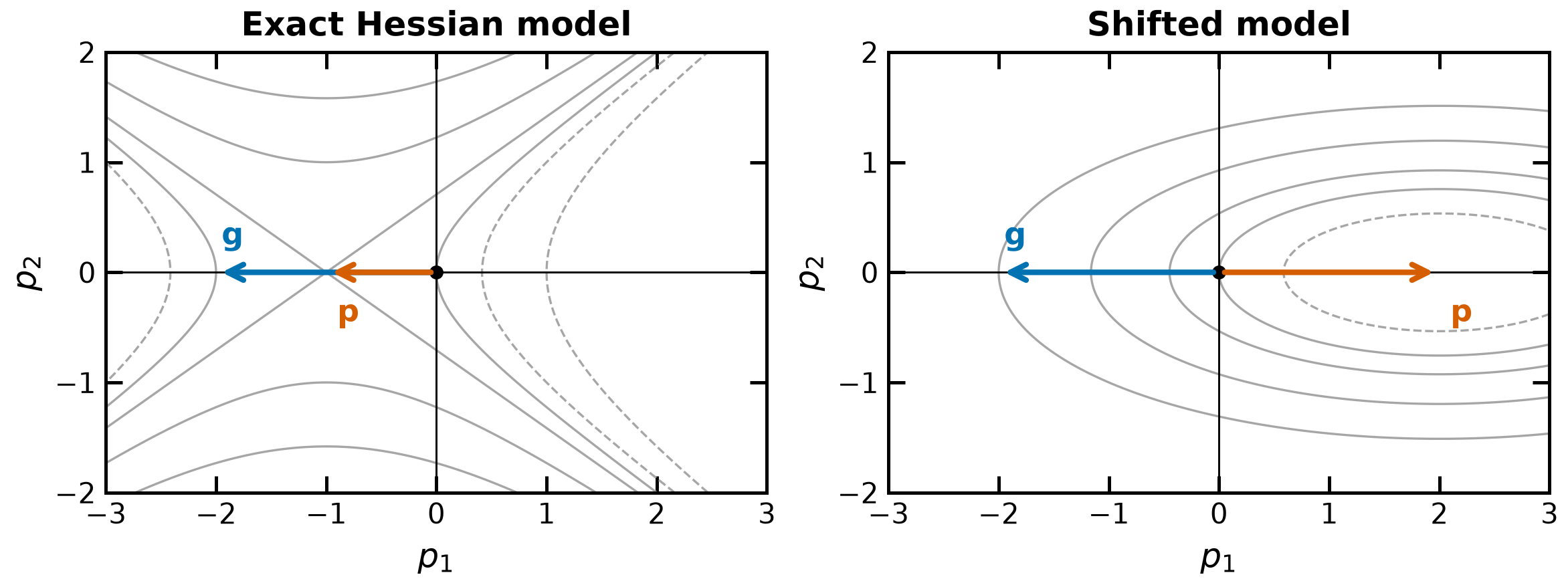
A Newton-type method uses a symmetric curvature model $\mathbf B^k$ and solves $\mathbf B^k\mathbf p^k=-\nabla f(\mathbf x^k)$. A positive-definite model gives a descent direction when the gradient is nonzero; an accepted update is $\mathbf x^{k+1}=\mathbf x^k+\alpha_k\mathbf p^k$. Unit-step modified Newton takes $\alpha_k=1$, but positive definiteness alone does not guarantee that this full step decreases the actual objective.

The examples below retain deliberate SR1 breakdowns. The detailed reference sections at the end explain the secant, signed update, curvature safeguards, and conditional rates. Biegler (2010), Algorithm 3.1 and §3.2, pp. 40–42.

For a differentiable objective and a nonzero gradient, a symmetric positive-definite model gives a descent direction. If its eigenvalues satisfy $0<m\le\lambda_j(\mathbf B)\le M$ for all $j$, the inverse Rayleigh bound gives

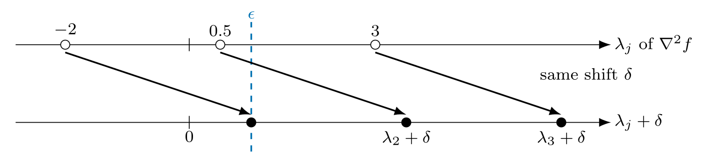
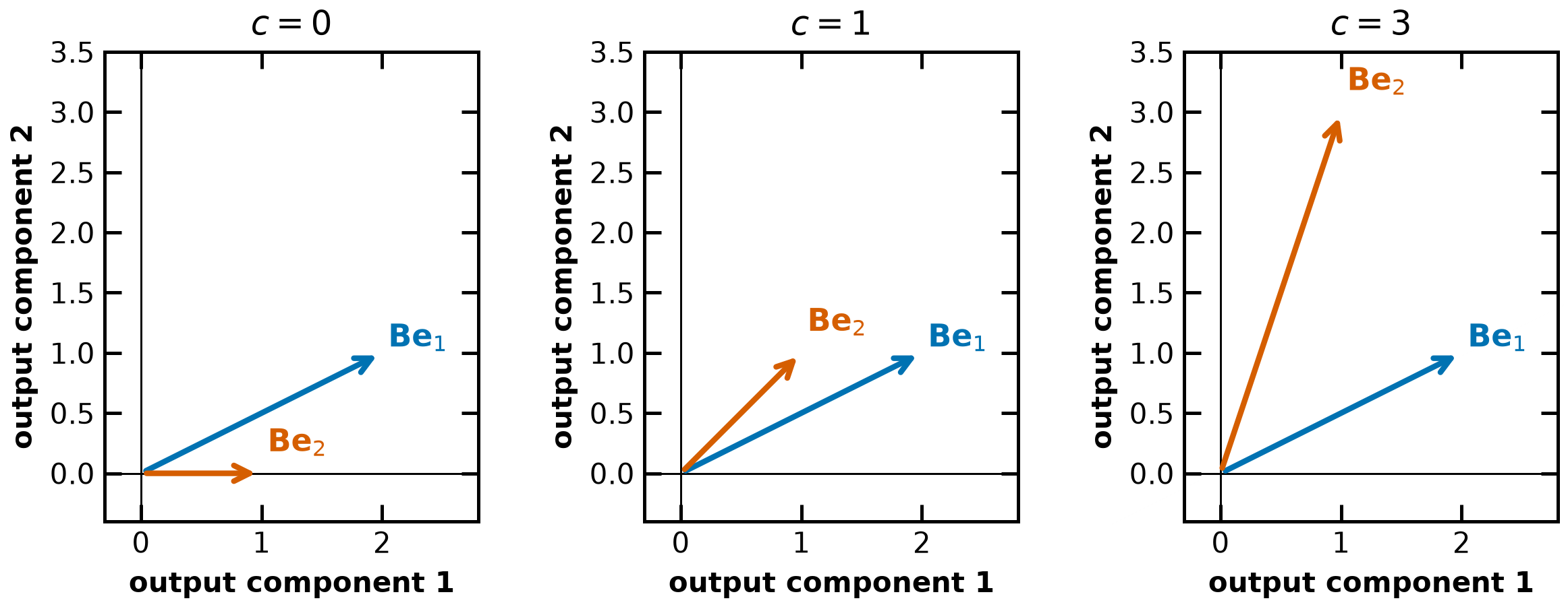
This proves a negative initial slope. Differentiability gives $f(\mathbf x+\alpha\mathbf p)-f(\mathbf x)=\alpha\mathbf g^T\mathbf p+o(\alpha)$, so sufficiently small positive steps decrease the objective. A full step can still overshoot. A scalar eigenvalue shift changes each eigenvalue by the same amount while preserving the eigenvectors. To enforce a floor $\epsilon>0$, the smallest nonnegative shift is $\delta=\max(0,\epsilon-\lambda_{\min})$. The diagram shows the shift geometry; the classroom example computes the shift from the original spectrum and the floor.

SR1 update is one way to approximate $\mathbf{B}^k$.

Library of helper functions¶

Symmetric Rank 1 (SR1) Update¶

Test Case: Simple quadratic program¶

Near solution¶

Consider $\mathbf{x}_0 = [-0.1, 0.2]^T$

Far from solution¶

Consider $\mathbf{x}_0 = [-100, 500]^T$

Activity/Discussion¶

• Does the number of iterations depend on the starting point for this problem?

• How many iterations are needed for Newton’s method to converge for a positive definite quadratic program using exact second derivative information?

• Why does the SR1 update not converge to the true Hessian?

Test Case: Example 2.19¶

Biegler’s two-variable test problem is

with $u=x_1-0.8$, $v=x_2-(a_1+a_2u^2(1-u)^{1/2}-a_3u)$, $\alpha=-b_1+b_2u^2(1+u)^{1/2}+b_3u$, and $\beta=c_1v^2(1-c_2v)/(1+c_3u^2)$. We use $\mathbf{a}=(0.3,0.6,0.2)$, $\mathbf{b}=(5,26,3)$, and $\mathbf{c}=(40,1,10)$.

The reported solution is $\mathbf{x}^*=(0.7395,0.3144)$ with $f(\mathbf{x}^*)=-5.0893$. The cells below recompute it rather than relying on the printed result. (Biegler, Example 2.19, p. 30.)

$\mathbf{x}_0$ somewhat near solution¶

Consider:

$\mathbf{x}_0$ far from solution¶

Consider:

Activity/Discussion¶

• Classify each candidate solution.

• Is the SR1 approximation always positive definite?

Broyden update with Cholesky factorization¶

As part of Algorithms Homework 3, you will adapt this example and implement the BFGS (Broyden-Fletcher-Goldfarb-Shanno) update formula.

You may decide to use the Cholesky factorization of $\mathbf{B}^{k}$,

to make your BFGS update more efficient. (This is not required). Let’s see how to do Cholesky factorization with SciPy.

Reference: secant measurements and signed SR1¶

Use Euclidean vector norms and their induced matrix norm unless a weighted norm is specified.

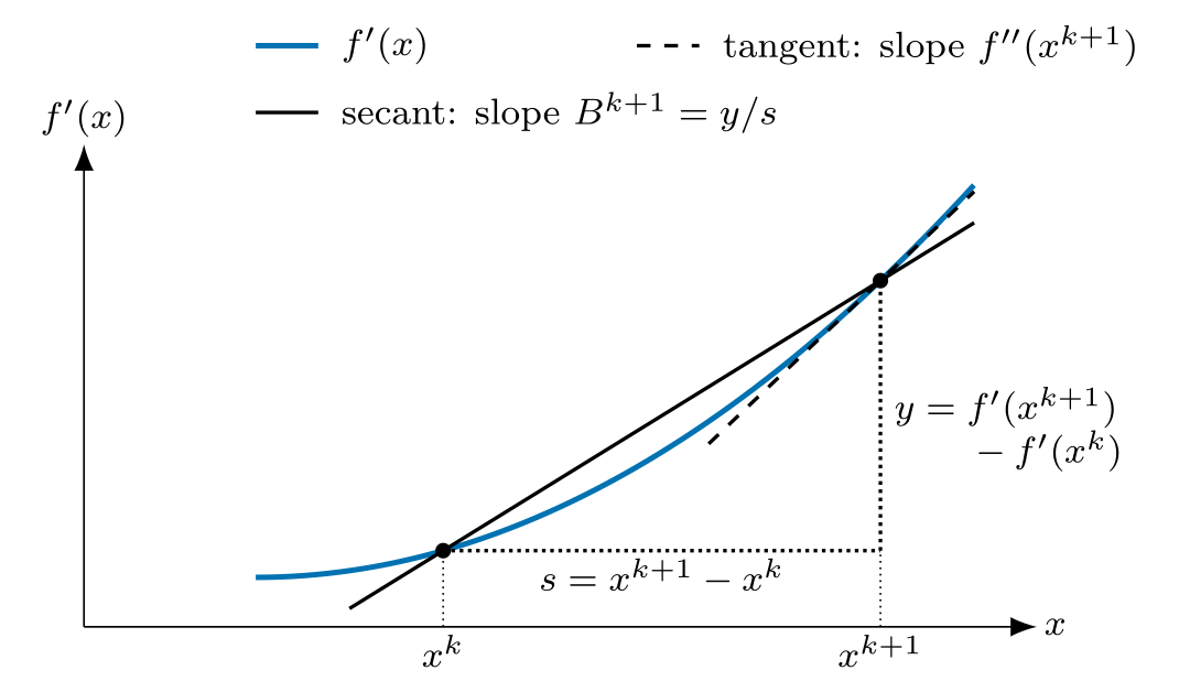
For a nonzero accepted displacement, $\mathbf s=\mathbf x^{k+1}-\mathbf x^k$ and $\mathbf y=\nabla f(\mathbf x^{k+1})-\nabla f(\mathbf x^k)$. For $f\in C^2(D)$ on an open $D$ containing the full segment $\{\mathbf x^k+t\mathbf s:0\le t\le1\}$, the componentwise FTC gives the exact identity

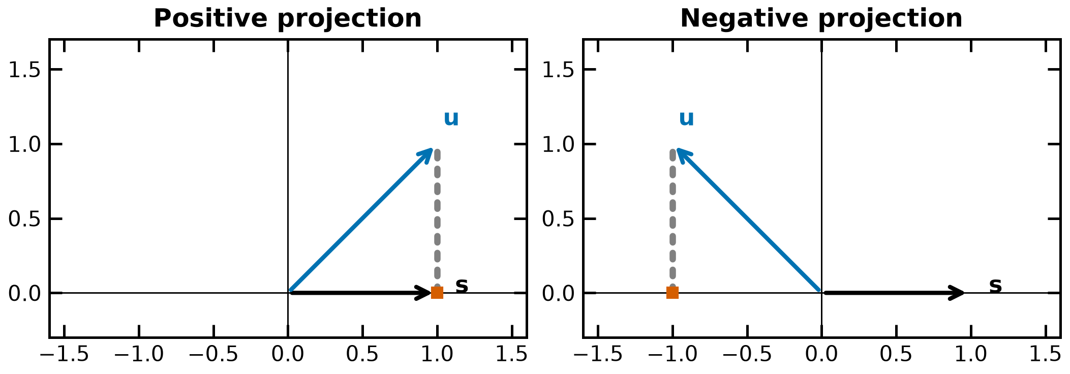
motivates $\mathbf B^{k+1}\mathbf s=\mathbf y$. It fixes the action on one direction, not every matrix entry. A symmetric $n\times n$ matrix has $n(n+1)/2$ free entries and a nonzero secant gives $n$ independent scalar equations. For example, $\mathbf s=\mathbf e_1$, $\mathbf y=(2,1)^T$ gives $\mathbf B^+=\begin{bmatrix}2&1\\1&c\end{bmatrix}$ with free $c$; positive definiteness adds $c>1/2$.

For $\mathbf u=\mathbf y-\mathbf B\mathbf s$, signed SR1 is

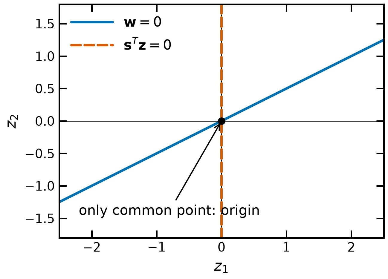
It has the form $\mathbf B+\sigma\mathbf w\mathbf w^T$ with $\sigma=\operatorname{sign}(\mathbf u^T\mathbf s)$ and $\mathbf w=\mathbf u/\sqrt{|\mathbf u^T\mathbf s|}$. A formula using only $+\mathbf w\mathbf w^T$ cannot represent negative denominators. Multiplying by $\mathbf s$ cancels the denominator and gives $\mathbf B^+\mathbf s=\mathbf B\mathbf s+\mathbf u=\mathbf y$.

To see why the zero-denominator case is an obstruction, suppose a nonzero symmetric rank-one correction $\sigma\mathbf w\mathbf w^T$ satisfies $\sigma\mathbf w(\mathbf w^T\mathbf s)=\mathbf u\ne0$. Then $\mathbf u$ is parallel to $\mathbf w$ and $\mathbf w^T\mathbf s\ne0$, so $\mathbf u^T\mathbf s=\sigma(\mathbf w^T\mathbf s)^2\ne0$. Thus $\mathbf u\ne0$ with $\mathbf u^T\mathbf s=0$ cannot be repaired by that rank-one form.

There are three cases: if $\mathbf u=0$, keep the existing matrix; if $\mathbf u\ne0$ but $\mathbf u^T\mathbf s=0$, no symmetric rank-one secant correction exists; if the denominator is small but nonzero, a large correction can amplify errors. Nocedal and Wright’s scale-aware safeguard accepts only if

Biegler gives the alternative threshold $|\mathbf u^T\mathbf s|\ge C_1\|\mathbf s\|^2$. Neither test enforces a positive sign; SR1 can represent indefinite curvature. A trust-region method can use that curvature, whereas a basic line-search step requires a descent direction.

Direction coverage also matters for recovering a Hessian. The precise nonlinear SR1 result uses uniform linear independence and its other convergence/safeguard hypotheses, not merely a different-looking sequence of steps. See Nocedal and Wright, Theorem 6.2, p. 149. Biegler’s short independence remark on p. 43 should be read with those hypotheses.

Sources: Biegler (2010), Eqs. (3.8)–(3.10), pp. 42–43; Nocedal and Wright (2006), §6.2, Eqs. (6.24) and (6.26), pp. 144–149.

Reference: BFGS, curvature safeguards, and implementation alternatives¶

With $\mathbf B\succ0$, $\mathbf s\ne\mathbf0$ and $\mathbf s^T\mathbf y>0$,

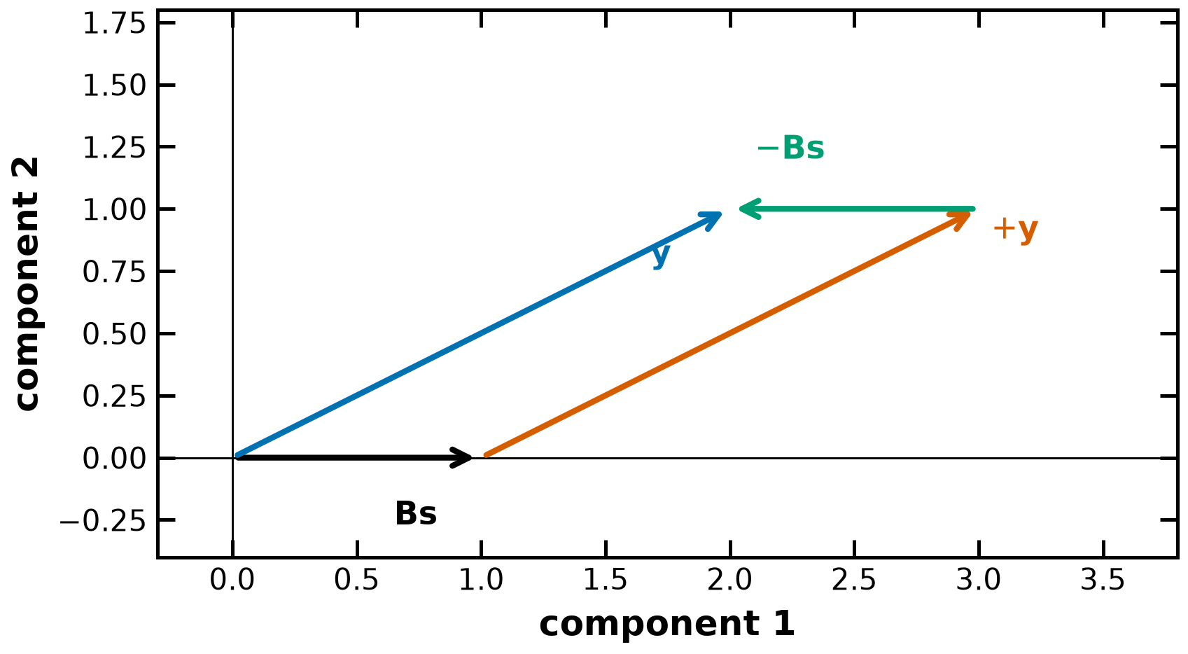
Multiplication by $\mathbf s$ gives $\mathbf B\mathbf s+\mathbf y-\mathbf B\mathbf s=\mathbf y$. The correction has rank at most two. The positive curvature condition is necessary for any positive-definite secant matrix: $\mathbf s^T\mathbf y=\mathbf s^T\mathbf B^+\mathbf s>0$.

A stronger quantitative test $\mathbf s^T\mathbf y\ge C_2\|\mathbf s\|^2$ can reject small positive curvature as well as zero or negative curvature. It does not, by itself, bound the matrix norm. With $\mathbf B=\mathbf I$, $\mathbf s=\mathbf e_1$, and $\mathbf y=(1,a)^T$, the scalar test is always $\mathbf s^T\mathbf y=1$, but

has an arbitrarily large largest eigenvalue as $|a|$ grows. Additional bounds on measurements and updates matter.

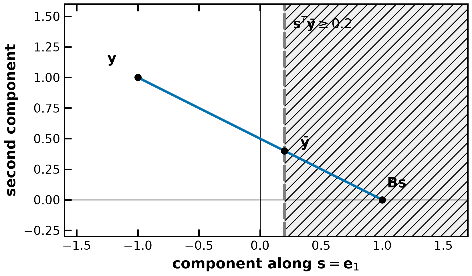
Powell damping. Let $b=\mathbf s^T\mathbf B\mathbf s>0$ and choose $\beta\in(0,1)$, commonly 0.2. Define $\bar{\mathbf y}=\theta\mathbf y+(1-\theta)\mathbf B\mathbf s$. Taking

makes $\mathbf s^T\bar{\mathbf y}\ge\beta b$; in the second case equality holds. The update then fits the damped measurement, not the original secant. The prepared picture below shows the interpolation and the permitted curvature half-space.

Inverse form. For $\mathbf H=\mathbf B^{-1}$, $\rho=1/(\mathbf s^T\mathbf y)$,

For any nonzero $\mathbf z$, write $\mathbf w=(\mathbf I-\rho\mathbf y\mathbf s^T)\mathbf z$. Then

If the second term is zero, $\mathbf w=\mathbf z\ne0$, so the first term is positive. Otherwise the second term is positive. This proves positive definiteness without an eigenvalue decomposition. In exact arithmetic the inverse update equals the inverse of the direct BFGS update.

A dense inverse update still stores $O(n^2)$ numbers and its matrix-vector step costs $O(n^2)$; avoiding a solve is not avoiding a matrix. A Cholesky-factor update is another option: update the factor and use triangular solves instead of refactorizing a full new matrix. Finite precision still matters. For the existing Hilbert-matrix conditioning demonstration, see Linear Algebra Review and SciPy Basics, section D2. The example is not duplicated here. Positive definiteness maintained algebraically does not by itself establish safe conditioning in floating point.

Weighted least-change characterizations distinguish the updates: an appropriate weighted Frobenius formulation for the Hessian gives DFP; the corresponding inverse formulation gives BFGS. The norm and weighting hypotheses are essential (Nocedal and Wright, Eqs. (6.9)–(6.17), pp. 138–140). The broader Broyden family and its parameterization are discussed by Al-Baali, Spedicato and Maggioni (2014), pp. 942–943; BFGS is the zero-parameter member in their convention.

Sources: Biegler (2010), Eqs. (3.18)–(3.21), pp. 44–45, and the errata for Eq. (3.23) if using its alternative rank-two vectors; Nocedal and Wright (2006), pp. 137–141; Dennis and Schnabel (1996), Lemma 9.2.1, p. 199, and Eq. (9.2.10), p. 201. These are mathematical reference formulas; the BFGS programming exercise above remains an exercise.

Reference: directional accuracy and superlinear convergence¶

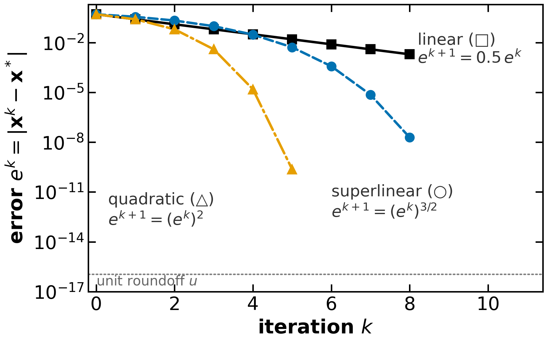
For a nonterminated convergent sequence $\mathbf x^k\to\mathbf x^*$ with $e_k=\|\mathbf x^k-\mathbf x^*\|>0$, Q-superlinear convergence means

Equivalently, $e_{k+1}/e_k\to0$. Finite termination requires no quotient. Linear and quadratic rates have their primary definitions in the Newton reference.

Let $f\in C^2(D)$ on an open neighborhood $D$ of $\mathbf x^*$, $\nabla f(\mathbf x^*)=0$, and $\nabla^2f(\mathbf x^*)\succ0$. Suppose unit-step iterates converge to $\mathbf x^*$, with symmetric positive-definite $\mathbf B^k$, $\mathbf B^k\mathbf p^k=-\mathbf g^k$ and nonzero errors/steps before termination. Superlinear convergence is equivalent to

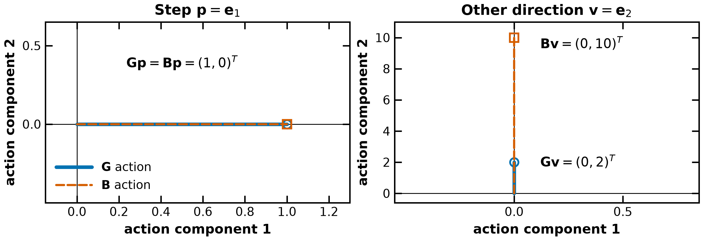
Using $\nabla^2f(\mathbf x^*)$ instead gives the same limit by Hessian continuity. The condition concerns the directions used. For $\mathbf G=\operatorname{diag}(1,2)$, $\mathbf B=\operatorname{diag}(1,10)$ and $\mathbf p=\mathbf e_1$, the directional error is zero despite $\|\mathbf B-\mathbf G\|=8$.

Proof mechanism. Write $\mathbf e_k=\mathbf x^k-\mathbf x^*$, $\mathbf G^k=\nabla^2f(\mathbf x^k)$ and $\mathbf p_N^k=-(\mathbf G^k)^{-1}\mathbf g^k$. Hessian continuity and nondegeneracy give a bounded inverse and $\mathbf e_k+\mathbf p_N^k=o(\|\mathbf e_k\|)$. A Lipschitz Hessian strengthens this to $O(\|\mathbf e_k\|^2)$, but that stronger assumption is unnecessary for the equivalence.

Subtracting the two solves gives

Under directional accuracy, the difference is $o(\|\mathbf p^k\|)$. Hence

Since $\|\mathbf p^k\|\le\|\mathbf e_k\|+\|\mathbf e_{k+1}\|$, rearranging for $\eta_k<1$ gives

Conversely, superlinear convergence gives $\mathbf p^k=-\mathbf e_k+o(\|\mathbf e_k\|)$ and thus $\|\mathbf p^k\|/\|\mathbf e_k\|\to1$. Subtracting the Newton-step remainder then gives $\mathbf p^k-\mathbf p_N^k=o(\|\mathbf e_k\|)$. Multiply by the bounded $\mathbf G^k$ and divide by $\|\mathbf p^k\|$ to recover directional accuracy. Finite termination is handled separately; the displayed ratios describe a nonterminated sequence.

A strict minimum alone is insufficient. For $f(x)=x^4$ with nonzero iterates, exact Newton has $B^k=f''(x^k)$, so its directional error is identically zero, yet $x^{k+1}=2x^k/3$ is only linear. Its limiting Hessian is zero. This exposes the missing nondegeneracy hypothesis in an unqualified reading of Biegler’s Theorem 3.1; Nocedal and Wright’s Theorem 3.7 states it explicitly.

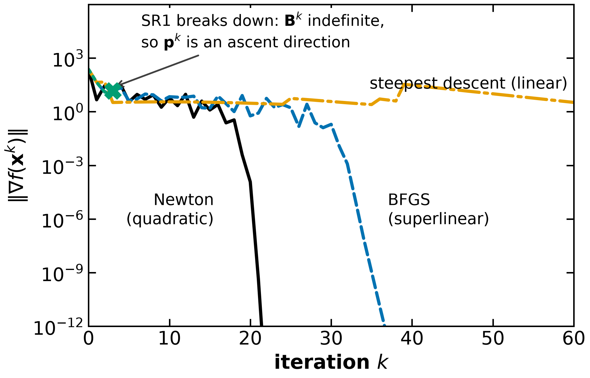
For standard BFGS, the local superlinear theorem assumes convergence, a nondegenerate minimizer, the bound $\|\nabla^2f(\mathbf x)-\nabla^2f(\mathbf x^*)\|\le L\|\mathbf x-\mathbf x^*\|$ near $\mathbf x^*$ for some $L>0$, summable iterate errors, and the specified line-search/update framework. Wolfe searches test the unit step first and use a sufficient-decrease parameter strictly below $1/2$ when invoking the unit-step admissibility result. A finite gradient-norm plot does not prove those assumptions or a convergence rate. The shared Rosenbrock comparison below is one numerical experiment; its unmodified SR1 run deliberately stops on an ascent direction.

Sources: Nocedal and Wright (2006), Theorems 3.6–3.7, pp. 46–47; Assumption 6.2, p. 156, and Theorem 6.6, p. 158; Biegler (2010), Theorems 3.1–3.2, pp. 42 and 44, read with the explicit nondegenerate-minimum hypothesis.

Reference: storage and derivative-acquisition costs¶

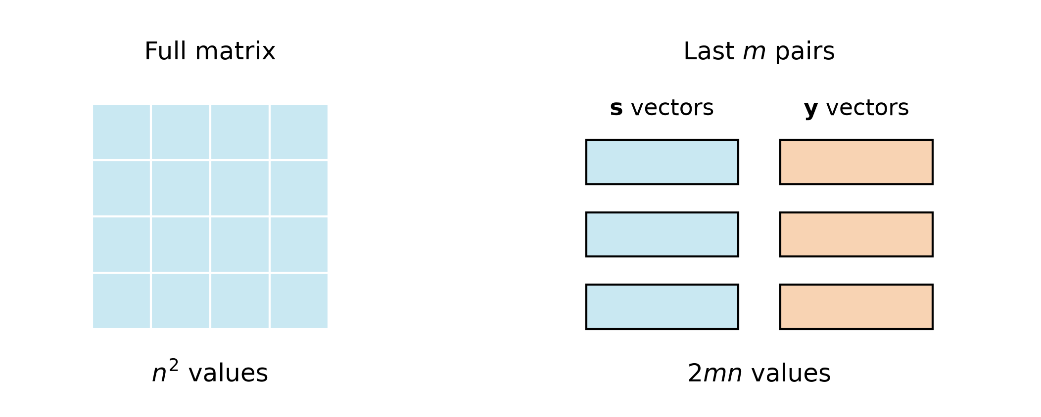
Full dense BFGS stores $n^2$ values. Fixed-memory L-BFGS retains $m$ recent secant pairs, or $2mn$ values, plus workspace and base scaling. Its two-loop recursion computes the inverse action without forming an $n\times n$ matrix (Nocedal and Wright, Algorithm 7.4, pp. 177–178). At float64 precision, $n=10^6$, $m=10$ means 8 TB for one dense matrix versus 160 MB for the pairs, in decimal units. This is storage accounting, not a timing benchmark.

Discarding pairs means fixed-memory L-BFGS does not inherit the full BFGS superlinear theorem. Linear-rate results for limited memory impose additional smoothness, curvature and algorithm hypotheses; memory size alone establishes no universal rate. See Liu and Nocedal (1989), Algorithm 2.1, p. 506, and Theorem 7.1, p. 524, with the discussion on p. 526.

When only function values are available, derivative cost depends on the stencil and reuse policy. Forward differences reuse $f(\mathbf x)$ and require $n+1$ distinct points for a gradient. A complete forward second-difference Hessian also needs $\mathbf x+2h\mathbf e_i$ and $\mathbf x+h\mathbf e_i+h\mathbf e_j$ for $i<j$:

Including the reused points gives $1+2n+n(n-1)/2$ evaluations, or 861 at $n=40$. A central Hessian stencil uses $1+2n^2$ distinct points, or 3201 at $n=40$; its mixed entries use four sign combinations per pair. These counts assume a dense Hessian, shared points, and one common step size; sparsity, automatic derivatives, constraints, noise and domain restrictions change the practical choice. The earlier rough $n^2/2$ estimate was an order-of-growth comparison, not an exact call count.

BFGS avoids Hessian acquisition, but finite-difference gradients can have an error floor that prevents the exact-derivative asymptotic theorem from applying. The notebook’s intentionally nonfinite-derivative examples remain useful checks of domain restrictions.

Additional reading: Nocedal and Wright (2006), §8.1, pp. 195–203, on derivative approximation; Biegler (2010), §3.3, pp. 42–46, on quasi-Newton implementation. Factorization/error demonstrations are kept in the existing linear-algebra reference pages rather than copied here.

Shared Rosenbrock experiment: complete settings and outcomes¶

The handout comparison uses the existing canonical figure implementation. Its model is

The derivatives used by the experiment are

All methods use the same wolfe_step routine: test $\alpha=1$ first, halve the trial value as needed, with $c_1=10^{-4}$ and $c_2=0.9$, and at most sixty trial reductions. The run records the gradient norm, uses threshold 10^-11 and at most sixty accepted steps. On an exhausted search this demonstration routine returns its final trial; that returned value is not automatically a Wolfe certificate. These are finite experiment settings, not the hypotheses of an unconditional convergence theorem.

Newton uses the exact Hessian, adding $(10^{-8}-\lambda_{\min}+10^{-3})\mathbf I$ if $\lambda_{\min}<10^{-8}$. BFGS begins with $\mathbf B^0=\mathbf I$ and updates only if $\mathbf s^T\mathbf y>10^{-12}$. SR1 also starts from $\mathbf I$, permits either denominator sign, and stops if $|\mathbf u^T\mathbf s|<10^{-14}$; it has no curvature repair. Before searching, the implementation rejects a nonnegative slope for its BFGS/SR1 solve. Steepest descent uses $\mathbf p=-\mathbf g$.

The stored plot history floors values at 10^-16 to support logarithmic display; it does not assert an exact derivative value of 10^-16. The shared SR1 run’s negative-denominator update creates indefinite curvature (eigenvalues approximately -642 and 6); the next slope is approximately +0.26, so the descent-based routine rejects that direction. The norm trace remains finite and does not certify a minimum or an asymptotic rate. Source code, settings and this table are available together so the comparison can be reproduced without changing the implementation’s ownership.